Introduction
Pharmacists are specialized health professionals with a Doctor of Pharmacy (PharmD) degree. Pharmacists are generally viewed as medication dispensing specialist, but they also monitor for potential drug-drug interactions, provide vaccinations, manage therapy for patients with chronic disease, and in some states, provide and deliver healthcare directly to patients. As the role of the pharmacist expands, the demand also has increased.
There has been a lot of research to understand the pharmacist labor market. In the early 2000s, reports indicated that there was a pharmacist shortage, which was fueled by the growing number of the senior citizen population and increased number of prescriptions.[1–3] This concern of a pharmacist labor market shortage, which was unable to meet the demand of a growing Medicare population, led to an increase in the number of Doctor of Pharmacy Schools in the United States from 80 in 2000 to approximately 140 in 2020.[4]
However, pharmacy school enrollment has been dwindling, which threatens the labor market supply. For instance, the number of applications to pharmacy schools dropped by 36% from 2012 to 2021.[5] This has led to some pharmacy school closures in recent years.[6,7] Further, the California Board of Pharmacy reported staffing levels at community pharmacies were dangerously low and could threaten patient care and safety.[8]
Microeconomic theory can provide some insights into the evolving pharmacy labor market. By using simple supply and demand curves, we can illustrate how these factors can impact the wages and quantity of pharmacists in the labor market.
Supply and Demand
The pharmacist labor market can be explained by the demand needed for their services and the number of available pharmacists in the workforce. It can also be explained by the supply of pharmacists currently in the market or entering the market.
Demand can be due to the expanding role of the pharmacist to provide innovative healthcare to their community, the growing senior citizen population, and the rise in prescriptions ordered and dispensed. Demand for pharmacist can also increase due to their evolving roles as practitioners.
Likewise, the supply of pharmacists in the workforce will depend on several factors such the number of new pharmacists entering the market (e.g., pharmacy school graduates) and the current supply that are already in the workforce. The supply of pharmacists will also be impacted by the number who retire or burnout and pursue other activities such as administrative roles.
We can use simple supply and demand curves to illustrate how the market (e.g., wages and quantity) can be impacted by things like a decrease in the enrollment and graduation of pharmacy students, the shrinking number of pharmacists due to retirement or leaving the workforce due to burnout, evolving role of pharmacists, and the increased number of senior citizens enrolled in Medicare.
Wages are important because this can incentive individuals to pursue a pharmacist career. If the wage is high enough, they are incentivized to enroll into a pharmacy school and become a pharmacist. However, if the wages are too low, then individuals are less likely to pursue a career in pharmacy. Likewise, firms will need to pay higher wages for pharmacists if there is a shortage and high demand for them in the market.
Simple example
In this simple illustration, the supply and demand curves are plotted along the wage (W) and quantity (Q) axes (Figure 1).
Figure 1. Simple demand and supply curves.
We can think of there being two players in this pharmacist labor market: Firms (employers) and pharmacists (employees). Pharmacies (e.g., firms/employers) have a need to hire pharmacist to deliver healthcare services, and pharmacists (employees) have a need for pharmacies to hire their labor. The demand and supply curves provide a visual approach to determine the ideal wage and quantity of pharmacists in the market.
The supply curve is upward sloping. As the wage of the pharmacist increases, there is an incentive to increase the quantity of pharmacists in the market. Individuals will go to pharmacy school and complete their training to become pharmacists. Likewise, pharmacy schools may increase enrollment or new pharmacy schools may open to meet the demand.
The demand curve is downward sloping. As the wage of the pharmacist decreases, there is very little to no incentive to become a pharmacist, thus, the quantity of pharmacists decreases. Conversely, if there is a high demand for pharmacists, then the firms will pay a higher wage in order to incentivize individuals to enter the pharmacist workforce.
The point where the supply and demand curves intersect is the equilibrium point. This is where the equilibrium wage (W*) and the equilibrium quantity (Q*) are determined. At the equilibrium wage W*, there should be an equilibrium quantity (Q*) of pharmacists in the labor market.
There are several assumptions we have to make with this simple example. First, this is a perfectly competitive market. This means that there are many firms or employers who will hire pharmacists. Second, market forces determine the wages in the pharmacist labor market. This means that pharmacists (employees) and firms (employers) are wage takes (not wage setters). Lastly, there is perfect information in the sense that both the firm and pharmacist know what the wages and quantity needed are or should be in the market.
With those things in place, we can see how the market can impact the wages and quantity of pharmacists in the workforce.
Factors that affect supply
It’s clear that the supply of pharmacists in the market will depend on the number of graduates and the current rate of pharmacist who retire. But there are other factors that can impact the supply of pharmacist in the labor market. For instance, pharmacists may work part-time thereby reducing the number of available pharmacists for the workforce. Pharmacists may also take on other non-patient care roles such as administration. Low enrollment and school closures can also affect the quantity of pharmacist in the market. Further, increased student debt may dis-incentivize individuals to pursue a career as a pharmacist.
When these factors occur, there is a shift in the supply curve to the left (Figure 2). This shift (S -> S') changes the equilibrium wage (W*) and quantity (Q*) of pharmacists to be higher and lower, respectively. As the supply of pharmacists in the labor market decreases, then the market will respond by setting a higher wage (W') but at a lower quantity (Q') of pharmacists. Alternatively, firms are willing to pay a higher wage for pharmacists due to a decrease in the labor supply.

Figure 2. Supply curve shifts to the left due to a shortage.
Conversely, there could a surplus of pharmacists in the workforce, which means that there are so many pharmacists that firms don’t need them. Alternatively, the large quantity of pharmacists shifts the supply curve to the right (S -> S''). This is illustrated in Figure 3. When the supply curve shifts to the right, the wage of the pharmacist becomes lower (W'') at the new quantity of pharmacists (Q'') that are hired by the firm. Having a lot of pharmacists is good for the firms since they can hire more at a lower wage. But this will disincentive individuals from pursuing a career in pharmacy.

Figure 3. Supply curve shifts to the right due to a surplus.
Factors that affect demand
But what about the factors that affect the demand of pharmacists in the workforce? How will that impact the wage and quantity?
Let’s consider a scenario where the senior citizen population is increasing and there is a need for pharmacists to educate them on their medications. Pharmacies are expecting a large number of Medicare Patients to also enroll in their Medication Therapy Management (MTM) plans where the pharmacist will be their main healthcare contact and provider. The expanding role of pharmacists and the increasing number of patients both contribute to the demand of pharmacists. This has an impact of the demand curve and shifts this to the right, D -> D'. Figure 4 illustrates the shift in the demand curve to the right where the wage of the pharmacist has increased to W' and the quantity hired has increased to Q'. In other words, firms are paying higher wages for pharmacist to fill critical roles in their pharmacies, which results in more pharmacists being hired to meet the increase in demand.

Figure 4. Demand curve shifts to the right due to an increase in the demand for pharmacists.
However, the demand or need for pharmacists can decrease due to market forces. The evolution of artificial intelligence and robotics may decrease the demand of pharmacists. Should this scenario occur, the demand for pharmacists will decrease, which is represented by a shift in the demand curve to the left (D -> D''). Figure 5 illustrates the impact that a decrease in the demand curve will have on the wage and quantity of the pharmacist in the workforce. As the demand curve shifts to the left, the wage (W'') is lower and the quantity (Q'') of pharmacists is also lower. This means that firms are going to hire less pharmacists at a lower wage due to a decrease in the demand.
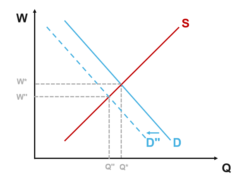
Figure 5. Demand curve shifts to the left due to a decrease in the demand for pharmacists.
Simultaneous shifts in the supply and demand
So far, we only looked at the effects that supply and demand would have on the pharmacy labor market independently of each other. But what is both the supply and demand are affected at the same time? What would happen to the pharmacy labor market in terms of wages and quantity hired?
Let’s consider a scenario where there is a shortage of pharmacists in the labor market, but the demand has increased due to an increasing number of senior citizens enrolled in Medicare (Figure 6). This would cause the supply curve to shift to the left (S -> S''') and the demand curve to shift to the right (D -> D'''). This would result in firms hiring more pharmacists (Q''') at a higher wage (W''').

Figure 6 illustrates what would have if there was a shortage of pharmacists and the demand increased.
We can consider the opposite effect where the demand of pharmacists decreases (or shifts to the left) and the supply increases (or shifts to the right). This would result in a depression in wages and a small increase in the quantity of pharmacists being hired (Figure 7). Firms will hire slightly more pharmacists at depressed wages due to a simultaneous decrease in demand and an increase in the supply of pharmacists in the workforce. I think of this as a worst-case scenario for the pharmacist profession.

Figure 7. Impact of decreased demand and increased supply of pharmacists in the workforce.
But that’s not all!
These shifts in the supply and demand curves are predictions. What if the shifts are greater?
Let’s consider an example where both the supply and demand curves have shifts that are greater than the examples above. In Figure 8, the supply curve shifts to the left in an extreme manner (e.g., a large number of pharmacists are leaving the workforce), and the demand curve shifts to the right in an extreme manner (e.g., the need for pharmacists has increased dramatically due to an increase in the senior citizen population). The wage (W''') has gone up dramatically and the supply (Q''') is now lower than original equilibrium quantity (Q*). Compare this to Figure 6 where the supply (Q''') was greater than the original equilibrium quantity (Q*).

Figure 8. Impact of both the supply and demand curves are ambiguous depending on the amount of the shifts.
This demonstrates to us that when both the supply and demand curves shift, we really don’t know what’s going to happen. Our predictions will depend on how much these curves shift and in what direction. To understand the effects of both the supply and demand curves of pharmacists shifting, we will need data.
Conclusions
Using simple illustrations of the supply and demand curves, we can visualize how the market would react to changes in the demand and supply of pharmacists in the workforce. We have to assume that the pharmacist labor market is in perfect competition. However, in the real-world, that doesn’t always occur. For example, studies have evaluated the impact of consolidation of (large retail chain) pharmacies that could control the market and force pharmacists to accept the wages they offer (monopsony).[9,10] This can violate the assumption of a pharmacist labor market being in perfect competition and seriously disadvantage pharmacists from not being able to negotiate fair wages. Moreover, when both the supply and demand curves shift, the effects on wages and quantity of pharmacists in the workforce is ambiguous; we will need data to understand what will happen to the pharmacist labor market. Regardless, by using these simple methods, we can start to understand how markets should behave in ideal conditions and when to identify when these markets are failing us, thereby requiring some policy intervention to make things more fair.
References
1. Knapp KK, Quist RM, Walton SM, Miller LM. Update on the pharmacist shortage: national and state data through 2003. Am J Health Syst Pharm. 2005;62(5):492-499. doi:10.1093/ajhp/62.5.492
2. Knapp KK, Livesey JC. The Aggregate Demand Index: measuring the balance between pharmacist supply and demand, 1999-2001. J Am Pharm Assoc (Wash). 2002;42(3):391-398. doi:10.1331/108658002763316806
3. Taylor TN, Knapp KK, Barnett MJ, Shah BM, Miller L. Factors affecting the unmet demand for pharmacists: state-level analysis. J Am Pharm Assoc (2003). 2013;53(4):373-381. doi:10.1331/JAPhA.2013.12130
4. Brown DL. Years of Rampant Expansion Have Imposed Darwinian Survival-of-the-Fittest Conditions on US Pharmacy Schools. Am J Pharm Educ. 2020;84(10):ajpe8136. doi:10.5688/ajpe8136
5. Pharmacy College Application Service. 2021-2022 - PharmCAS Applicant Data Report. Accessed December 17, 2023. https://connect.aacp.org/discussion/pharmcas-applicant-data-for-2021-2022
6. Harsa C. Husson University to close its pharmacy school. newscentermaine.com. February 17, 2025. Accessed June 22, 2025. https://www.newscentermaine.com/article/news/education/husson-university-pharmacy-school-program-university-of-new-england-students-maine/97-665e64a5-ecb9-44ea-a1ed-187e6fb495a7
7. American Association of Colleges of Pharmacy. Pharmacy Schools Are Essential to Meeting Growing Demand for Pharmacists’ Services. Accessed June 22, 2025. https://www.aacp.org/article/pharmacy-schools-are-essential-meeting-growing-demand-pharmacists-services
8. California Board of Pharmacy. Pharmacy Workforce Survey, 2021. California Board of Pharmacy; 2021. Accessed December 18, 2023. https://www.pharmacy.ca.gov/meetings/agendas/2021/workforce_presentation.pdf
9. Farag E, Steinbaum M. A Retrospective Analysis of the Acquisition of Target’s Pharmacy Business by CVS Health: Labor Market Perspective. Published online November 25, 2023. doi:10.2139/ssrn.4644895
10. Bounthavong M. Despair and hope: Is the retail community pharmacy workforce in danger of becoming a monopsony labor market? J Am Pharm Assoc (2003). 2024;64(3):102039. doi:10.1016/j.japh.2024.02.012