Methods

Using inverse probability of treatment weights & Marginal structural models to handle time-varying covariates

BACKGROUND

When constructing regression models, there are two approaches to handling confounders: (1) conditional and (2) marginal approaches.(1) The conditional approach handles confounders using stratification or modeling (e.g., adding covariates to be regressed to the outcome). Whereas, the marginal approach uses weights to balance the confounders across treatment exposure levels.(1–5) In conventional regression models, the exposure is regressed to the outcome controlling for potential confounders. However, in longitudinal data, time-varying confounders can result in biased estimates of the model parameters if not properly adjusted. This gets more complicated when we have a time-varying exposure in the model to account for.

In panel data analysis or longitudinal data analysis, adjusting for time-varying exposure and time-varying confounders are critical to reducing bias. Additionally, there are time-dependent relationships between the confounders and exposure that need to be considered when adjusting for longitudinal regression models. In this article, we will focus on the marginal approach in terms of using the inverse probability of treatment weights fitted to a marginal structural model.

This article was published on RPubs with the corresponding R code using RMarkdown and can be located at this link.


TIME-DEPENDENT RELATIONSHIPS

In Figure 1, the time-dependent relationships between times 1 and 0 for the treatment variable are indicated by the arrows (We look at the relationships across two time points. In actual longitudinal data, there may be more than two time points to consider). Notice how the Outcome at time==0 is a confounder for the relationship between Exposure and Outcome at time==1.

Figure 1. Time-dependent relationships between the exposure and outcome variables.

Figure 1 - time-dependent relationships.png

Conventional methods to perform longitudinal data analysis such as linear mixed effects models and generalized estimating equations models are capable of handling time-varying covariates. However, in the case of a time-varying elements, the probability of treatment exposure is invariably different across time, which requires application of time-varying weights on the unit of analysis (e.g., individual subjects).

We can address this issue by applying inverse probability of treatment weights (IPTW) to the observations, which are then fitted to a marginal structural model (MSM).(4,5) IPTW are used to make the exposure at time 0 and 1 independent of the confounders that occur beforehand and allow us to generate a causal interpretation between the treatment exposure on the outcome.


DESCRIPTION OF METHODS

IPTW are weights assigned to each observation across time conditioned on the previous exposure history, which are then multiplied to generate a single weight for a subject. Similar to conventional propensity score estimation, IPTW is generated using either a logit or probit model that regresses covariates to a treatment group (exposure) variable. With IPTW, the previous exposure history is incorporated to the propensity score estimation, which is time-varying.

Standardized weights in a longitudinal setting are estimated as

 
Figure 2 - sw equation.png
 

where A is the exposure for subject i at time t_ij (time points range starting at k = 0 to k=j). The numerator contains the probability of the observed exposure at each time point (a_ik) conditioned on the observed exposure history of the previous time point (a_ik-1) and the observed non-time varying covariates (v_i). The denominator contains the probability of the observed exposure at each time point conditioned on the observed exposure history of the previous time point (a_ik-1), the observed time-varying covariates history at the current time point (c_ik), and the non-time varying covariates (v_i).

In standardized weights, the time-varying confounders are captured in the denominator but not in the numerator. However, the non-time varying (also known as fixed-time) covariates are captured in both the numerator and denominator to stabilize the weights. Using stabilized weights is preferable to non-standardized weights, which are not discussed in this article.

Some statistical software are unable to handle time-varying weights; hence, a single weight for each individual needs to be estimated. Once the standardized weights for subject i at time t_ij are calculated, a single weight is estimated by multiplying all the standardized weights across the time points, which is then applied in a marginal structural model for subject i.

There are several key assumptions that must be made in order for IPTW methods to generate causal interpretation between the exposure and outcome (Thoemmes and colleagues provides a detailed explanation in their paper)(5):

1) No unmeasured confounding

2) Positivity

3) Correct specification of the IPTW


Given these assumptions are met, using IPTW fitted to an MSM can yield causal inference between the treatment exposure and outcome. This method is flexible enough where it can be applied to a linear mixed effects model, generalized estimating equation model, and survival model. Gerhard and colleagues used this approach (marginal structural Cox model) to estimate the treatment effects of antihypertensive therapy in a non-randomized trial.(6) Hernan and colleagues used a marginal structural Cox proportional hazard model to estimate the treatment effect of zidovudine and Pnuemocystis carinii therapy on survival of HIV-positive homosexual males in a non-randomized trial.(4)  


MOTIVATING EXAMPLE

This article will use CRAN R program statistical software to perform the IPTW fitted to an MSM. We will use the data that was simulated using the following R commands.

#set seed to replicate results
set.seed(12345)

#define sample size
n <- 2000

#define confounder c1 (gender, male==1)
male <- rbinom(n,1,0.55)

#define confounder c2 (age)
age <- exp(rnorm(n, 3, 0.5))

#define treatment at time 1
t_1 <- rbinom(n,1,0.20)

#define treatment at time 2
t_2 <- rbinom(n,1,0.20)

#define treatment at time 3
t_3 <- rbinom(n,1,0.20)

#define depression at time 1 (prevalence = number per 100000 population)
d_1 <- exp(rnorm(n, 0.001, 0.5))

#define depression at time 2 (prevalence = number per 100000 population)
d_2 <- exp(rnorm(n, 0.002, 0.5))

#define depression at time 3 (prevalence = number per 100000 population)
d_3 <- exp(rnorm(n, 0.004, 0.5))

#define tme-varying confounder v1 as a function of t1 and d1
v_1 <- (0.4*t_1 + 0.80*d_1 + rnorm(n, 0, sqrt(0.99))) + 5

#define tme-varying confounder v2 as a function of t1 and d1
v_2 <- (0.4*t_2 + 0.80*d_2 + rnorm(n, 0, sqrt(0.55))) + 5

#define tme-varying confounder v3 as a function of t1 and d1
v_3 <- (0.4*t_3 + 0.80*d_3 + rnorm(n, 0, sqrt(0.33))) + 5

#put all in a dataframe and write data to harddrive to use later in e.g. SPSS
df1 <- data.frame(male, age, v_1, v_2, v_3, t_1, t_2, t_3, d_1, d_2, d_3)

write.table(round(df1,11),"data1.csv", row.names = FALSE, quote = FALSE)

A little data manipulation was done to make treatment in the following period equal to 1 if the previous period was also equal to 1. In other words, E[Treatment=1, time=1 | Treatment=1, time=time-1]. Age was rounded to the nearest whole number. You can download the *CSV file here.

The dataset contains variables for id, male, age, treatment (t), outcome (d), time-varying covariate (v), and time. Exploring the dataset set, we see the structure as:

 
Figure 4 - dataset.png
 

There are 2000 individuals with three repeated measures of the t, v, and d variables. The t variable represents the Treatment exposure, which is time-varying. The v variable represents an arbitrary time-varying covariate. And the d variable is the outcome (dependent) variable, which is also time-varying. Non-time varying covariates include the age at baseline and the gender of each individual.


LONGITUDINAL DATA ANALYSIS APPROACH

Generalized estimating equations (GEE) were constructed to evaluate the impact of the treatment (t) on the outcome (d) and to handle the time-varying covariate (v) in the panel dataset. Since the outcome was a continuous variable, a generalized linear Gaussian family with identity link was used. Auto-regressive (AR1) correlation structure was selected since this was a time series (panel) data; we expected the correlation to decay as the outcome values were farther away from the time of interest. 

We will need the following packages:

geepack

survey

ipw

reshape

deplyr


The following R code was used to generate the IPTW and fitted to a MSM using GEE.

#######################################################################
# Install the required packages
#######################################################################
library(geepack)
library(survey)
library(ipw)
#library(foreign)
#library(multcomp)
#library(gee)
library(reshape)
library(dplyr)

#######################################################################
#Estimate ipw weights (time-varying)
#######################################################################
# estimate inverse probability weights (time-varying) using a logistic regression
w <- ipwtm(
  exposure = t,
  family = "binomial",
  link = "logit",
  numerator = ~ factor(male) + age,
  denominator = ~ v + factor(male) + age,
  id = id,
  timevar=time,
  type="first",
  data = data_long_sort)
summary(w$ipw.weights)

iptw = w$ipw.weights


# Add the iptw variable onto a new dataframe = data2.
data2 <- cbind(data_long_sort, iptw)

#######################################################################
# Plot the stabilized inverse probability weights
#######################################################################
ipwplot(weights = data2$iptw, 
        timevar = data2$time, 
        binwidth = 0.5,
        main = "Stabilized weights", 
        xaxt = "n",
        yaxt = "n")

#######################################################################
# confint.geeglm function (to generate 95% CI for the geeglm())
#######################################################################
confint.geeglm <- function(object, parm, level = 0.95, ...) {
  cc <- coef(summary(object))
  mult <- qnorm((1+level)/2)
  citab <- with(as.data.frame(cc),
                cbind(lwr=Estimate-mult*Std.err,
                      upr=Estimate+mult*Std.err))
  rownames(citab) <- rownames(cc)
  citab[parm,]
}


#######################################################################
# GEE model #1.1 - GEE with cluster robust SE (no IPTW)
#######################################################################
gee.bias <- geeglm(d~t + time + factor(male) + age + cluster(id),
                    id=id,
                    data=data2, 
                    family=gaussian("identity"), 
                    corstr="ar1")
summary(gee.bias)
confint.geeglm(gee.bias, level=0.95)

#######################################################################
# GEE model #2 - IPTW fitted to MSM with clustered robust SE
#######################################################################
gee.iptw <- geeglm(d~t + time + factor(male) + age + cluster(id),
                   id=id,
                   data=data2, 
                   family=gaussian("identity"), 
                   corstr="ar1", 
                   weights=iptw)
summary(gee.iptw)
confint.geeglm(gee.iptw, level=0.95)

We compared the findings from the convention GEE model without IPTW to the GEE model incorporating IPTW (Table). The differences are significant. In the standard GEE model, the treatment (t) is associated with a reduction in the outcome (d) by 0.012 units with a 95% confidence interval (CI) of -0.020 and 0.045, which is not statistically significant. Conversely, in the GEE model incorporating IPTW, the treatment (t) is associated with a reduction in the outcome (d) by 0.071 units with a 95% CI of -0.104 and -0.038, which is statistically significant. 

Figure 5 - model comparisons.png


CONCLUSIONS

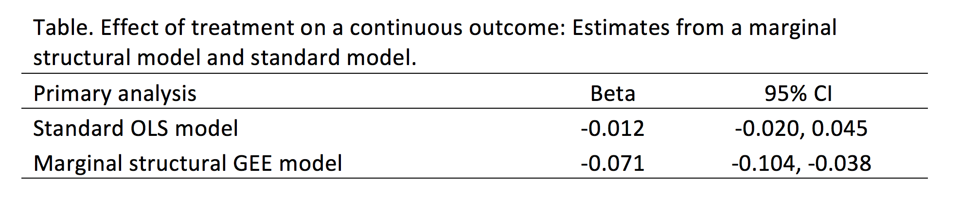
Based on our findings, the IPTW fitted to a MSM (GEE model) resulted in a statistically significant reduction in the treatment on the outcome that would not have otherwise been captured in the conventional GEE model. Given that there are time-varying covariates (especially with the treatment variable), IPTW fitted to a MSM may yield important differences that would otherwise be unidentified with conventional methods. However, it is critical that all assumptions regarding the IPTW method are satisfied prior to accepting the model’s results.


REFERENCES

1. Williamson T, Ravani P. Marginal structural models in clinical research: when and how to use them? Nephrol Dial Transplant. 2017 Apr 1;32(suppl_2):ii84–90.

2. Robins JM, Hernán MA, Brumback B. Marginal structural models and causal inference in epidemiology. Epidemiol Camb Mass. 2000 Sep;11(5):550–60.

3. Hernán MA, Hernández-Díaz S, Robins JM. A structural approach to selection bias. Epidemiol Camb Mass. 2004 Sep;15(5):615–25.

4. Hernán MA, Brumback B, Robins JM. Marginal Structural Models to Estimate the Joint Causal Effect of Nonrandomized Treatments. J Am Stat Assoc. 2001 Jun 1;96(454):440–8.

5. Thoemmes F, Ong AD. A Primer on Inverse Probability of Treatment Weighting and Marginal Structural Models. Emerg Adulthood. 2016 Feb 1;4(1):40–59.

6. Gerhard T, Delaney JA, Cooper-DeHoff RM, Shuster J, Brumback BA, Johnson JA, et al. Comparing marginal structural models to standard methods for estimating treatment effects of antihypertensive combination therapy. BMC Med Res Methodol. 2012 Aug 6;12:119.

Estimating marginal effects using Stata Part 1 – Linear models

BACKGROUND

Regression models provide unique opportunities to examine the impact of certain predictors on a specific outcome. These predictors’ effects are usually isolated using the model coefficients adjusting for all other predictors or covariates. A simple linear regression model with a single predictor x_i is represented as

 
fig1.png
 

where y_i denotes the outcome (dependent) variable for subject i, beta0 denotes the intercept, beta1 is the model coefficient that denotes the change in y due to a 1-unit change in x, and epsilon_i is the error term for subject i.

A 1-unit increase in x is associated with some change in the outcome y. This finding may explain predictor variable x’s impact on outcome variable y, but it doesn’t not tell us the impact of a representative or prototypical case.

The marginal effect allows us to examine the impact of variable x on outcome y for representative or prototypical cases. For example, Stata’s margins command can tell us the marginal effect of body mass index (BMI) between a 50-year old versus a 25-year old subject.

There are three types of marginal effects of interest:

1.       Marginal effect at the means (MEM)

2.       Average marginal effect (AME)

3.       Marginal effect at representative values (MER)

Each of these marginal effects have unique interpretations that will impact how you examine the regression results. (We will focus on the first two, since the third one is an extension of the AME.) The objective of this tutorial is to review these marginal effects and understand their interpretations through examples using Stata.


MOTIVATING EXAMPLE

We will use the Second National Health and Nutrition Examination Survey (NHANES) data from the 1980s, which can be found in Stata’s library using the following command:

use http://www.stata-press.com/data/r15/nhanes2.dta

Table 1 summarizes the characteristics of the NHANES population.

fig2.png


ADJUSTED PREDICTIONS

Adjusted prediction for a regression model provides the expected value of an outcome y conditioned on x assuming all other things are equal. In other words, this is the effect of the predictor variable x regressed to outcome variable y adjusting or controlling for other covariates. Therefore, if you were comparing the effect of a 1-unit increase in age to the BMI, then you could compare this across all patients who are equally White, Black, or Others.

Example 1

A simple linear regression model can capture the incremental effect of age on body mass index. For example, the impact of age on body mass index (BMI) can be represented as a linear regression:

 
FIG3.png
 

where BMI_1  is the body mass index for individual i, beta0 denotes the intercept (or BMI when AGE=0), beta1 denotes the change in BMI for each 1-unit increase in Age for individual i, and episilon_i denotes the error term for individual i. (The unit of BMI is kg/m^2).

The Stata command to perform a simple linear regression:

regress bmi age

The corresponding regression output is:

fig4.png

In this regression output example, the predictor of interest is AGE. The _cons parameter denotes the coefficient beta0 otherwise known as the intercept; therefore, a subject with AGE = 0 has a BMI that is 23.2 kg/m^2. (Although this is unrealistic, we will ignore this for now.) The impact AGE has on the BMI is denoted by the slope parameter beta1, which is the change in BMI due to a 1-unit change in Age. In this example, the a 1-unit increase in Age is associated with a 0.05 kg/m^2 increase in BMI.

If we wanted to know the difference in BMI between a 50-year old and 25-year old, we need to estimate the adjusted prediction, which estimates the difference in the outcome based on some user-defined values for the x variables.

To estimate the adjusted predicted BMI for a 50-year old, we used the following equation:

 
fig5.png
 

which is 25.7 kg/m^2. We can do this using the following Stata command:

di _b[_cons] + 50*_b[age]
25.655896

Similarly, we can estimate the adjusted predicted BMI for a 25-year old:

 
fig6.png
 

which is 24.4 kg/m^2.

The difference between these two is:

25.655896 - 24.433991 = 1.2 kg/m^2. 

Therefore, the difference in BMI between a 50-year old and 25-year old is on average 1.2 kg/m^2. This seems like a tedious process, but let’s see how we can make this exercise simpler using Stata’s margins command.

We can use Stata’s margins command to estimate the adjusted predicted BMI for a 50-year old and 25-year old:

margins, at(age=(25 50))

Figure 2. Stata’s margins command output for adjusted prediction of BMI for a 50-year old and 25-year old.

fig7.png

Example 2

We use a linear regression with other independent variables to illustrate the complexity of having other covariates adjusted in the model.

The regression model has the structure:

 
fig8.png
 

where  is the body mass index for individual i, beta0 is the intercept (or BMI when AGE=0), beta1 is the change in BMI for each 1-unit increase in Age for individual i, beta2 denotes the change in BMI for a female relative to a male, beta3 denotes the change in BMI due to contrasts in race categories (White, Black, and Other), and  is the error term for individual i. (The unit of BMI is kg/m^2).

For this example, RACE will be included into the regression model as a dummy variable using the following Stata command:

regress bmi age i.race i.sex

The corresponding regression output is:

fig9.png

The following are interpretations of the regression output.

A 1-unit increase in age is associated with a BMI increase of 0.05 kg/m^2 adjusting for race and sex or all things being equal.

Blacks are associated with a BMI increase of 1.4 kg/m^2 adjusting for age and sex compared to Whites.

Others are associated with a BMI decrease of 1.2 kg/m^2 adjusting for age and sex compared to Whites.

Females are associated with a BMI increase of 0.03 kg/m^2 adjusting for age and race.

If we wanted to know the adjusted prediction for a 50-year old and 25-year old, we can use the margins command:

margins, at(age=(25 50)) atmeans vsquish

The output is similar to Example 1 but there are some differences.

fig10.png

The atmeans option captures the “average” sample covariates. In our example, the mean proportion of females is 0.525, males is 0.475, Whites is 0.876, Blacks is 0.105, and Others is 0.019. Therefore, the adjusted predictions for 50-year old and 25-year old’s BMI is conditioned on the “average” values of the covariates in the model. This may not make sense because an individual subject can’t be 0.525 female and 0.475 male. Fortunately, we have other ways to address this with the marginal effect.


MARGINAL EFFECT

Marginal effect with the margins command generates the change in the conditional mean of outcome y with respect to a single predictor variable x. In other words, this is the partial effect of x on the outcome y for some representative or prototypical case. Usually this is obtained by performing a first-order derivative of the regression expression:

 
fig11.png
 

where the partial effect of the expected value of y condition on x is the first order derivative of the expected value of y condition on x with respect to x.

The representative or prototypical case can be the mean, observed, or a user defined case.


MARGINAL EFFECT OF THE MEAN (MEM)

MEM is the partial effect of on the dependent variable (y) conditioned on a regressor (x) after setting all the other covariates (w) at their means. In other words, MEM is the difference in x’s effect on y when all other covariates (RACE and FEMALE) are at their mean.

Let’s revisit the linear regression model but with the dummy variables included:

 
FIG12.png
 

In the output the beta1 = 0.0493881.

Getting the partial effect with respect to Age at the means for the other covariates, we use the following command:

regress bmi age i.race i.sex
FIG13.png
margins, dydx(age) atmeans vsquish
FIG14.png

Interpretation: For a subject who is average on all characteristics, the marginal change of a 1-unit increase in age is a 0.049 increase in the BMI.

We can also look at the MEM at different ages (e.g., 25 and 50 years):

margins, dydx(age) at(age=(25 50)) atmeans vsquish

This command performs the MEM for 25- and 50-year old subjects with their covariates set at the population mean. We interpret the results as the effect of age at different values of age at the average values of the other covariates.

The MEM should be:

fig15.png

The effect of age at 25 and 50 years old is an increase of 0.05 years. Notice that the MEM for 25- and 50-year olds are the same (MEM = 0.0493881). This is because the model is a linear regression. For every incremental increase in age, the incremental increase in the BMI is 0.0493881 given the other covariates are set at the mean.

To illustrate, we can manually perform this operation using the information above. Recall that the linear regression model with the dummy variables is represented as:

 
fig16.png
 

BMI for a 25-year old subject at the mean = intercept + 25*(beta1) + (mean of Black)*(beta2) + (mean of Other)*(beta3) + (mean of Female)*(beta4) = 24.42243 kg/m^2.

BMI for a 25-year old subject at the mean = 23.0528 + 25*(0.0493881) + .1049174*(1.382849) + .0193218*(-1.2243) + .5251667*(.025702) = 24.42243 kg/m^2, which is the same as the value presented in the adjusted prediction output.

Why are these the same? The linear regression is predictable in terms of the slope coefficients. Therefore, an incremental increase in predictor variable x will have the same incremental marginal increase in outcome variable y. When you apply the MEM to non-linear models, the slopes are no longer linear and will change based on varying levels of the continuous predictor x.


AVERAGE MARGINAL EFFECT (AME)

Unlike the MEM the average marginal effect (AME) doesn’t use the mean for the covariates when estimating the partial effect of the predictor variable x on the outcome variable y. Rather, the AME estimates the partial effect of the variable x on the outcome variable y for using the observed values for the covariates and then the average of that partial effect is estimated. In other words, the partial derivative is estimated with respect to x using the observed values for the other covariates (RACE and FEMALE), and then the average of that first-order derivative are averaged over the entire population to yield the AME. This is represented as:

 
ame figure.png
 

where the partial derivative of the estimated value of the outcome variable y with respect to x is conditioned on the values of covariates (w) for subject i over the entire population (N) and multiplied by beta_k (or the parameters of interest) .

Getting the partial effect with respect to Age at the observed values for the other covariates, we use the following command:

regress bmi age i.race i.sex

margins, dydx(age) asobserved vsquish
fig18.png

Interpretation: The average marginal effect of a 1-unit increase in age is a 0.049 increase in the BMI.

We can also look at the AME at different ages (e.g., 25 and 50 years):

margins, dydx(age) at(age=(25 50)) asobserved vsquish

This command performs the MEM for 25- and 50-year old subjects with their covariates set at the observed values. We interpret the results as the effect of age at different values of age at the observed values of the other covariates.

The AME should be:

fig19.png

The effect of age at 25 and 50 years old is an increase of 0.05 years. Notice that the AME for 25- and 50-year olds are the same (MEM = 0.0493881). Similar to the MEM, this is because the model is a linear regression. For every incremental increase in age, the incremental increase in the BMI is 0.0493881 given the other covariates are set at the observed values.


CONCLUSIONS

We see that the MEM and AME are exactly the same because of the linear model. The marginal effect of an increase in 1-unit of age is an increase in 0.05 kg/m^2 of the BMI. In the next part, non-linear models will be used to demonstrate that the MEM and AME are not equal.


REFERENCES

I used the following websites to help create this tutorial:

https://thomasleeper.com/margins/articles/Introduction.html

https://support.sas.com/rnd/app/ets/examples/margeff/index.html

https://www.ssc.wisc.edu/sscc/pubs/stata_margins.htm


I also used the following paper by Richard Williams:

Using the margins command to estimate and interpret adjusted predictions and marginal effects. The Stata Journal. 2012;12(2):308-331.

https://www.stata-journal.com/article.html?article=st0260