Linear spline (piecewise) models in Stata

I wrote a tutorial on how to construct linear spline (also known as piecewise) models using Stata, which has been uploaded to my RPubs site.

Previously, I have developed tutorial on using the linear spline method for interrupted time series analsyis with Stata. However, I did not properly go over the mkspline commands.

In this tutorial, I review the mkspline command and the marginal option to generate coefficients that could be interpreted as the slope within each segment or the change in slope between segments, respectively.

View fullsize

Interpreting regression models

I wrote a short explanation on how to interpret regression models.

I have posted this on RPubs, and the code is saved on my GitHub site.

View fullsize

R tutorials on confounding/interaction and linear regression model - Updates

Last year, I created several tutorials on how to use R for identifying confounding/interaction and visualizing linear regression models. I updated these tutorials recently to address some errors and mistakes. They have received new hyperlinks:

R tutorial on confounding and interactions using the epitool and epiR packages is located on my RPubs page here. The R Markdown code is located on my GitHub page here.

R tutorial on linear regression model is located on my RPubs page here. The R Markdown code is located on my GitHub page here.

View fullsize

View fullsize

Visualizing linear regression models using R - Part 2

I continue my previous blog post on visualizing linear regression models using R (link). Part 2 focuses on using visualization to assess whether the model’s residuals were associated with the predicted values and whether they are normally distributed.

The R Markdown code that I wrote to create this tutorial is located on my GitHub site (link).

You can find the tutorials on my RPubs site:

• Part 1 - Visualizing linear regression model using R (link)

• Part 2 - Visualizing linear regression model using R (link)

(NOTE: on 30 January 2022, I updated these tutorials and they can be found in my RPubs page here. The R Markdown code is saved on my GitHub page here.)

View fullsize

Visualizing linear regression models using R - Part 1

I wrote a tutorial on how to visualize linear regression models using R. In the tutorial I used the lm() command and the predict3d package to generate the models and visualize them using R. You can view the RPubs tutorial here. (NOTE: on 30 January 2022, I updated this tutorial and it can be found in my RPubs page here.) I created this tutorial using R Markdown, and the codes are available on my GitHub site (link).

View fullsize

View fullsize

Estimating marginal effects using Stata Part 1 – Linear models

BACKGROUND

Regression models provide unique opportunities to examine the impact of certain predictors on a specific outcome. These predictors’ effects are usually isolated using the model coefficients adjusting for all other predictors or covariates. A simple linear regression model with a single predictor x_i is represented as

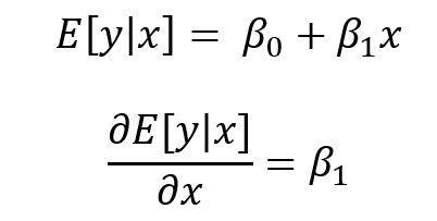
where y_i denotes the outcome (dependent) variable for subject i, beta0 denotes the intercept, beta1 is the model coefficient that denotes the change in y due to a 1-unit change in x, and epsilon_i is the error term for subject i.

A 1-unit increase in x is associated with some change in the outcome y. This finding may explain predictor variable x’s impact on outcome variable y, but it doesn’t not tell us the impact of a representative or prototypical case.

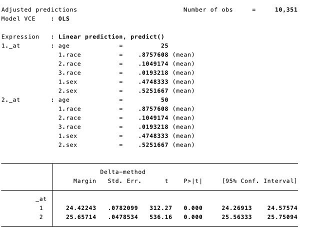
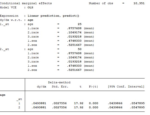
The marginal effect allows us to examine the impact of variable x on outcome y for representative or prototypical cases. For example, Stata’s margins command can tell us the marginal effect of body mass index (BMI) between a 50-year old versus a 25-year old subject.

There are three types of marginal effects of interest:

1.       Marginal effect at the means (MEM)

2.       Average marginal effect (AME)

3.       Marginal effect at representative values (MER)

Each of these marginal effects have unique interpretations that will impact how you examine the regression results. (We will focus on the first two, since the third one is an extension of the AME.) The objective of this tutorial is to review these marginal effects and understand their interpretations through examples using Stata.

 

MOTIVATING EXAMPLE

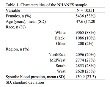
We will use the Second National Health and Nutrition Examination Survey (NHANES) data from the 1980s, which can be found in Stata’s library using the following command:

use http://www.stata-press.com/data/r15/nhanes2.dta

Table 1 summarizes the characteristics of the NHANES population.

 

ADJUSTED PREDICTIONS

Adjusted prediction for a regression model provides the expected value of an outcome y conditioned on x assuming all other things are equal. In other words, this is the effect of the predictor variable x regressed to outcome variable y adjusting or controlling for other covariates. Therefore, if you were comparing the effect of a 1-unit increase in age to the BMI, then you could compare this across all patients who are equally White, Black, or Others.

Example 1

A simple linear regression model can capture the incremental effect of age on body mass index. For example, the impact of age on body mass index (BMI) can be represented as a linear regression:

where BMI_1  is the body mass index for individual i, beta0 denotes the intercept (or BMI when AGE=0), beta1 denotes the change in BMI for each 1-unit increase in Age for individual i, and episilon_i denotes the error term for individual i. (The unit of BMI is kg/m^2).

The Stata command to perform a simple linear regression:

regress bmi age

The corresponding regression output is:

In this regression output example, the predictor of interest is AGE. The _cons parameter denotes the coefficient beta0 otherwise known as the intercept; therefore, a subject with AGE = 0 has a BMI that is 23.2 kg/m^2. (Although this is unrealistic, we will ignore this for now.) The impact AGE has on the BMI is denoted by the slope parameter beta1, which is the change in BMI due to a 1-unit change in Age. In this example, the a 1-unit increase in Age is associated with a 0.05 kg/m^2 increase in BMI.

If we wanted to know the difference in BMI between a 50-year old and 25-year old, we need to estimate the adjusted prediction, which estimates the difference in the outcome based on some user-defined values for the x variables.

To estimate the adjusted predicted BMI for a 50-year old, we used the following equation:

which is 25.7 kg/m^2. We can do this using the following Stata command:

di _b[_cons] + 50*_b[age]
25.655896

Similarly, we can estimate the adjusted predicted BMI for a 25-year old:

which is 24.4 kg/m^2.

The difference between these two is:

25.655896 - 24.433991 = 1.2 kg/m^2. 

Therefore, the difference in BMI between a 50-year old and 25-year old is on average 1.2 kg/m^2. This seems like a tedious process, but let’s see how we can make this exercise simpler using Stata’s margins command.

We can use Stata’s margins command to estimate the adjusted predicted BMI for a 50-year old and 25-year old:

margins, at(age=(25 50))

Figure 2. Stata’s margins command output for adjusted prediction of BMI for a 50-year old and 25-year old.

Example 2

We use a linear regression with other independent variables to illustrate the complexity of having other covariates adjusted in the model.

The regression model has the structure:

where  is the body mass index for individual i, beta0 is the intercept (or BMI when AGE=0), beta1 is the change in BMI for each 1-unit increase in Age for individual i, beta2 denotes the change in BMI for a female relative to a male, beta3 denotes the change in BMI due to contrasts in race categories (White, Black, and Other), and  is the error term for individual i. (The unit of BMI is kg/m^2).

For this example, RACE will be included into the regression model as a dummy variable using the following Stata command:

regress bmi age i.race i.sex

The corresponding regression output is:

The following are interpretations of the regression output.

A 1-unit increase in age is associated with a BMI increase of 0.05 kg/m^2 adjusting for race and sex or all things being equal.

Blacks are associated with a BMI increase of 1.4 kg/m^2 adjusting for age and sex compared to Whites.

Others are associated with a BMI decrease of 1.2 kg/m^2 adjusting for age and sex compared to Whites.

Females are associated with a BMI increase of 0.03 kg/m^2 adjusting for age and race.

If we wanted to know the adjusted prediction for a 50-year old and 25-year old, we can use the margins command:

margins, at(age=(25 50)) atmeans vsquish

The output is similar to Example 1 but there are some differences.

The atmeans option captures the “average” sample covariates. In our example, the mean proportion of females is 0.525, males is 0.475, Whites is 0.876, Blacks is 0.105, and Others is 0.019. Therefore, the adjusted predictions for 50-year old and 25-year old’s BMI is conditioned on the “average” values of the covariates in the model. This may not make sense because an individual subject can’t be 0.525 female and 0.475 male. Fortunately, we have other ways to address this with the marginal effect.

 

MARGINAL EFFECT

Marginal effect with the margins command generates the change in the conditional mean of outcome y with respect to a single predictor variable x. In other words, this is the partial effect of x on the outcome y for some representative or prototypical case. Usually this is obtained by performing a first-order derivative of the regression expression:

where the partial effect of the expected value of y condition on x is the first order derivative of the expected value of y condition on x with respect to x.

The representative or prototypical case can be the mean, observed, or a user defined case.

MARGINAL EFFECT OF THE MEAN (MEM)

MEM is the partial effect of on the dependent variable (y) conditioned on a regressor (x) after setting all the other covariates (w) at their means. In other words, MEM is the difference in x’s effect on y when all other covariates (RACE and FEMALE) are at their mean.

Let’s revisit the linear regression model but with the dummy variables included:

In the output the beta1 = 0.0493881.

Getting the partial effect with respect to Age at the means for the other covariates, we use the following command:

regress bmi age i.race i.sex

margins, dydx(age) atmeans vsquish

Interpretation: For a subject who is average on all characteristics, the marginal change of a 1-unit increase in age is a 0.049 increase in the BMI.

We can also look at the MEM at different ages (e.g., 25 and 50 years):

margins, dydx(age) at(age=(25 50)) atmeans vsquish

This command performs the MEM for 25- and 50-year old subjects with their covariates set at the population mean. We interpret the results as the effect of age at different values of age at the average values of the other covariates.

The MEM should be:

The effect of age at 25 and 50 years old is an increase of 0.05 years. Notice that the MEM for 25- and 50-year olds are the same (MEM = 0.0493881). This is because the model is a linear regression. For every incremental increase in age, the incremental increase in the BMI is 0.0493881 given the other covariates are set at the mean.

To illustrate, we can manually perform this operation using the information above. Recall that the linear regression model with the dummy variables is represented as:

BMI for a 25-year old subject at the mean = intercept + 25*(beta1) + (mean of Black)*(beta2) + (mean of Other)*(beta3) + (mean of Female)*(beta4) = 24.42243 kg/m^2.

BMI for a 25-year old subject at the mean = 23.0528 + 25*(0.0493881) + .1049174*(1.382849) + .0193218*(-1.2243) + .5251667*(.025702) = 24.42243 kg/m^2, which is the same as the value presented in the adjusted prediction output.

Why are these the same? The linear regression is predictable in terms of the slope coefficients. Therefore, an incremental increase in predictor variable x will have the same incremental marginal increase in outcome variable y. When you apply the MEM to non-linear models, the slopes are no longer linear and will change based on varying levels of the continuous predictor x.

AVERAGE MARGINAL EFFECT (AME)

Unlike the MEM the average marginal effect (AME) doesn’t use the mean for the covariates when estimating the partial effect of the predictor variable x on the outcome variable y. Rather, the AME estimates the partial effect of the variable x on the outcome variable y for using the observed values for the covariates and then the average of that partial effect is estimated. In other words, the partial derivative is estimated with respect to x using the observed values for the other covariates (RACE and FEMALE), and then the average of that first-order derivative are averaged over the entire population to yield the AME. This is represented as:

where the partial derivative of the estimated value of the outcome variable y with respect to x is conditioned on the values of covariates (w) for subject i over the entire population (N) and multiplied by beta_k (or the parameters of interest) .

Getting the partial effect with respect to Age at the observed values for the other covariates, we use the following command:

regress bmi age i.race i.sex

margins, dydx(age) asobserved vsquish

Interpretation: The average marginal effect of a 1-unit increase in age is a 0.049 increase in the BMI.

We can also look at the AME at different ages (e.g., 25 and 50 years):

margins, dydx(age) at(age=(25 50)) asobserved vsquish

This command performs the MEM for 25- and 50-year old subjects with their covariates set at the observed values. We interpret the results as the effect of age at different values of age at the observed values of the other covariates.

The AME should be:

The effect of age at 25 and 50 years old is an increase of 0.05 years. Notice that the AME for 25- and 50-year olds are the same (MEM = 0.0493881). Similar to the MEM, this is because the model is a linear regression. For every incremental increase in age, the incremental increase in the BMI is 0.0493881 given the other covariates are set at the observed values.

CONCLUSIONS

We see that the MEM and AME are exactly the same because of the linear model. The marginal effect of an increase in 1-unit of age is an increase in 0.05 kg/m^2 of the BMI. In the next part, non-linear models will be used to demonstrate that the MEM and AME are not equal.

REFERENCES

I used the following websites to help create this tutorial:

https://thomasleeper.com/margins/articles/Introduction.html

https://support.sas.com/rnd/app/ets/examples/margeff/index.html

https://www.ssc.wisc.edu/sscc/pubs/stata_margins.htm

I also used the following paper by Richard Williams:

Using the margins command to estimate and interpret adjusted predictions and marginal effects. The Stata Journal. 2012;12(2):308-331.

https://www.stata-journal.com/article.html?article=st0260