Truncated Axis

Communicating data effectively with data visualization - Part 4 (Time series)

Introduction

An important element of data visualization is to tell a story. To do that, we should have the end in mind. Namely, what is it you want to share with your audience?

Often, time series data can do this using some clever data visualization. Typically, this is presented on an XY plane where time is presented on the X-axis and the value of interest is presented on the Y-axis. We will not go into time series analysis, which involves a lot more than just plotting the data. However, we will go over the proper way in which to present your time series data visually.


Motivating example

We will use data from the National Health Expenditure Account (NHEA), which contains historical data on health expenditures in the U.S. from 1960 to 2016. The costs presented by the NHEA are properly adjusted for inflation. You can find the data at this link: https://www.cms.gov/Research-Statistics-Data-and-Systems/Statistics-Trends-and-Reports/NationalHealthExpendData/NationalHealthAccountsHistorical.html


Time series data

To visualize time series data, it is best to have increments of time that are equally spaced in the X-axis. We use Excel to illustrate these examples. Figure 1 illustrates the annual interval of national health expenditures ($ billions) in the United States from 1960 to 2016. The outcome (national health expenditure) is on the Y-axis and time (year) is on the X-axis. Notice that each time increment is one year and evenly spaced across the X-axis. This allows the eyes to intuitively see the changes across time in the U.S. national health expenditure.

Figure 1. National Healthcare Expenditure in the United States, 1960 to 2016.

Figure 1.png

What if the story is to see highlight health expenditures in the last decade? How would we do this?

First, we can use the same data and restrict the X-axis to 2007 to 2016 as in Figure 2.


Figure 2. National Health Expenditures in the United States, 2007 to 2016.

Screen Shot 2018-01-24 at 6.02.04 PM.png

Figure 2 doesn’t seem interesting. There is an increase in health expenditures from 2007 to 2016, but this doesn’t seem significant. However, there is a 45% increase from 2007 to 2016 in health expenditures ($2,295 billion to $3,337 billion). Figure 2 doesn’t convey this increase because there is a lot of white space between the lowest health expenditure value in 2007 and $0.

One way to illustrate the large increase in health expenditure is to truncate the Y-axis. In previous articles, we stressed that truncated axis can distort and trick the mind into seeing large differences where they don’t exist. However, this same technique can be used to make sure that differences that exist are not misinterpreted as not visually significant. According to Tufte:

In general, in a time-series, use a baseline that shows the data not the zero point. If the zero point reasonably occurs in plotting the data, fine. But don't spend a lot of empty vertical space trying to reach down to the zero point at the cost of hiding what is going on in the data line itself.[1]

In other words, time series data should focus on the area of the timeline that is interesting. The graphic should eliminate the white space and show the data horizontally for time series visuals.

Eliminating the white space and identifying the baseline value as $2,200 billion instead of $0 changes the figure as illustrated in Figure 3.


Figure 3. National Health Expenditures in the United States, 2007 to 2016.

Figure 3.png

Figure 3 illustrates the increase in national expenditure in the last decade better than Figure 2 and maintains the narrative that there was a visually significant increase.

Putting these concepts together (along with Tufte’s other principles), we can generate a similar figure using R (Figure 4). The R code is listed below.

# Plot trend - without truncation
library(lattice)
  
xyplot(y~x, 
       xlab=list(label="Year", cex=1.25),
       ylab=list(label="National Health Expenditures ($ Billions)", cex=1.25),
       main=list(lable="National Health Expenditure (2007 to 2016)", cex=2),
       par.settings = list(axis.line = list(col="transparent")),
       panel = function(x, y,...) { 
          panel.xyplot(x, y, col="darkblue", pch=16, cex=2, type="o")
          panel.rug(x, y, col=1, x.units = rep("snpc", 2), y.units = rep("snpc", 2), ...)})

Figure 4. National Health Expenditures in the United States, 2007 to 2016.

Figure 4 (darkblue).png

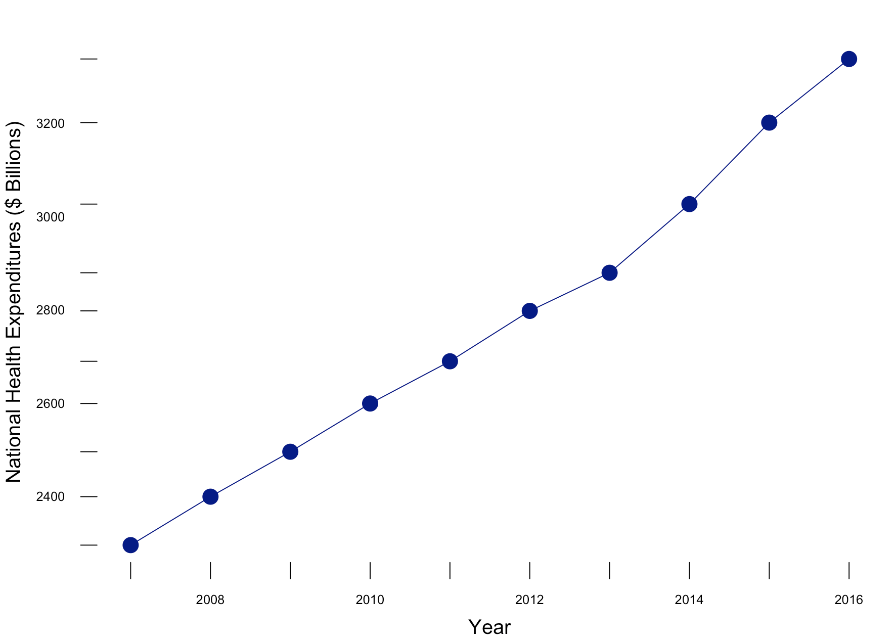
Figure 4 incorporates the use of Tufte’s principles on data-ink ratio and truncation on the y-axis to highlight the change in National Health Expenditure between 2006 go 2017.


Conclusions

With time series data, truncating the Y-axis to eliminate white space and show the data horizontally is appropriate when telling the story of what’s happening across time. Using zero as the baseline for the Y-axis is appropriate if it is reasonable. However, do not compromise the story by having the Y-axis extend all the way to zero if it doesn’t tell the story properly. Knowing when and how to truncate the Y-axis will help you explain to your audience the significance of a change across a specific period in time.


References

1. Edward Tufte forum: baseline for amount scale [Internet]. [cited 2018 Jan 14];Available from: https://www.edwardtufte.com/bboard/q-and-a-fetch-msg?msg_id=00003q

Communicating data effectively with data visualization – Part 3 (Truncated Axis and Area as Quantity)

Introduction

Data visualization is a powerful tool that allows us to use data to tell an engaging story. The narrative we present is enhanced by our data, especially when it is easily accessible and intuitive to understand. This is evident by the large amount of data visualization tools and galleries available throughout the internet. For example, Tableau Software hosts a data viz gallery that allows users to post their creations using their software. However, for most users, Microsoft Excel is the first tool they are exposed to when it comes to developing data visualizations for their business, school, and social projects.

Creating data visualization has its caveats. Improper data visualization can mislead, distort, and “lie,” which can result in poor decisions, loss of profit, and regret. In this blog, we will explore two of the most common distortion techniques that violate Tufte’s principles of graphical integrity: Truncated Axis and Area as Quantity.[1]


Motivating example

We will use data from the Medical Expenditures Panel Survey, which is a large-scale survey of households on health care resource use and spending in the United States. We will compare insurance status (Private, Public, Uninsured) between genders, which is summarized in Table 1. We will use Microsoft Excel to generate all our examples.

Table 1.png


Distortions

Data visualization has opened the door to increased misrepresentation of numbers. Interest groups and advocates will distort the data visualization to try and mislead or convince their audience of their arguments or narrative. Such techniques include using truncating axes and disproportionate sizes.

Let’s compare the difference in the proportion of males with public insurance to females with public insurance. In Figure 1, a bar chart is used to compare the proportion of males and females with access to public insurance. In Panel A, a truncated y-axis is used to distort the difference in the proportion of males and females with public insurance. The absolute difference is approximately 4%. However, Panel B, which uses a non-truncated y-axis, the perceived difference is not as great as that appearing in Panel A, despite having an absolute difference of 4%. Our mind perceives Panel A as having a greater difference; however, Panel B shows the same absolute difference of 4%, but does not illicit the same perception. This is supported by a study performed by Pandey and colleagues who reported that respondents rated the truncated bar chart as having a greater difference than the non-truncated bar chart.[2] It is our recommendation that a non-truncated y-axis is used when presenting data as a bar chart.

Figure 1. Comparisons of bar charts using a truncated y-axis (A) and a full y-axis (B).

Figure 1.png

Another distortion technique uses disproportionate sizes or “Area and Quantity” method. With this distortion, the values or quantitative data is not proportional to the area that represents it. Tufte argues that “the representation of numbers, as physically measured on the surface of the graph itself, should be directly proportional to the numerical quantities represented.”[1] In order words, the area used to represent the values or quantitative data should not be grossly exaggerated. Figure 2 illustrates how this principle is violated.

Figure 2. Proportion of males and females with public insurance using improper Area as Quantity.

Figure 2.png


In Figure 2, 27% of males have public insurance versus 31% of females. In terms of relative difference, females have a 15% greater proportion with public insurance compared to males per the equation: .

However, the area in Figure 2 has females with an area that is 96% greater than males, which is not reflective of the relative difference of 15%.

Figure 3 illustrates the correct Area as Quantity that reflect the relative difference between males and females with public insurance. We estimated the area of the circle for males and females and properly adjusted the sizes to reflect their relative differences. Now, the relative difference is not as great as previously illustrated. Instead, we have an accurate representation of the relative difference in having public insurance between males and females. We recommend estimated the area of a shape to reflect the relative difference between the groups with these types of data visualizations.

Figure 3. Proportion of males and females with public insurance using the proper Area as Quantity.

Figure 3.png

Conclusions

Distortions can mislead or convince an audience of a narrative that do not reflect the actual data. Developing data visualization that provides empirical support for your narrative should be accurate and honest. Fortunately, innocent mistakes like the examples above are easy to correct, especially when using programs like Microsoft Excel.


Notes

We calculated the area of the circle using Archimedes method where Area = pr^2 where p is the constant (p=3.14) and r is the radius of the circle.


References

1. Tufte ER. The Visual Display of Quantitative Information. Second. Cheshire, CT: Graphics Press, LLC.; 2001.

2. Pandey AV, Rall K, Satterthwaite ML, Nov O, Bertini E. How Deceptive Are Deceptive Visualizations?: An Empirical Analysis of Common Distortion Techniques [Internet]. In: Proceedings of the 33rd Annual ACM Conference on Human Factors in Computing Systems. New York, NY, USA: ACM; 2015. p. 1469–1478.Available from: http://doi.acm.org/10.1145/2702123.2702608