
BACKGROUND
In data visualization circles, the pie chart is considered an inefficient tool to convey parts of a whole. Edward Tufte often criticizes the use of the pie chart to display data visually stating that
“A table is nearly always better than a dumb pie chart; the only worse design than a pie chart is several of them, for then the viewer is asked to compare quantities located in spatial disarray both within and between charts.”[1]
The major reason why pie charts are disliked by data scientists and other pundits is due to the way our brain works. Mostly, we are good at judging things visually, but with pie charts, it is hard to distinguish the relative proportion of a slice to the whole. For example, can you tell the difference in proportions between the two pie charts below? Which one has more of component B?

Since it is challenging to identify the differences between the two pie charts, several alternatives exists to present the data accurately and effectively. In this article, we will discuss one such method using a waffle chart.
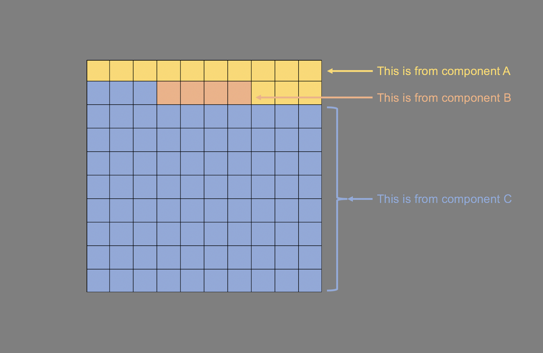
Waffle charts are grid-based visuals that have equal size blocks that convey parts of a whole accurately and efficiently. Some have called waffle charts the “square pie charts.” They are usually proportional and arranged in a 10 x 10 grid.

Colors can be used to distinguish the contribution of groups or categories to the whole where each square represents a percentage point totaling to 100.
Waffle charts are great at presenting data where you are describing the proportions or parts of a whole and should be used instead of pie charts.
MOTIVATING EXAMPLE
We will use the 2016 National Healthcare Expenditure dataset to illustrate the use of waffle charts. We will compare expenditures from the decades between 1965 and 2015.
You can download the data from the National Health Expenditures Accounts (NHEA) website:
The data provide the percentages of expenditures for different components spent on health for each decade from 1965 to 2015 (Table 1).
Table 1. National Health Expenditures from 1965 to 2015.

In the above table (we will start with 1965), 89% of Health Consumption Expenditures was due to Personal Health Care (83%), Government Administration And Net Cost Of Health Insurance (4%), and Government Public Health Activities (2%). The remainder was spent on Investments (11%). We have to estimate the cumulative percentage spent across the different categories to generate our waffle charts.
This is easily done by summing the individual components (Personal Health Care, Government Administration And Net Cost Of Health Insurance, Government Public Health Activities, and Investment) so that they will total 100 (Table 2).
Table 2. Cumulative values of the individual expenditures.

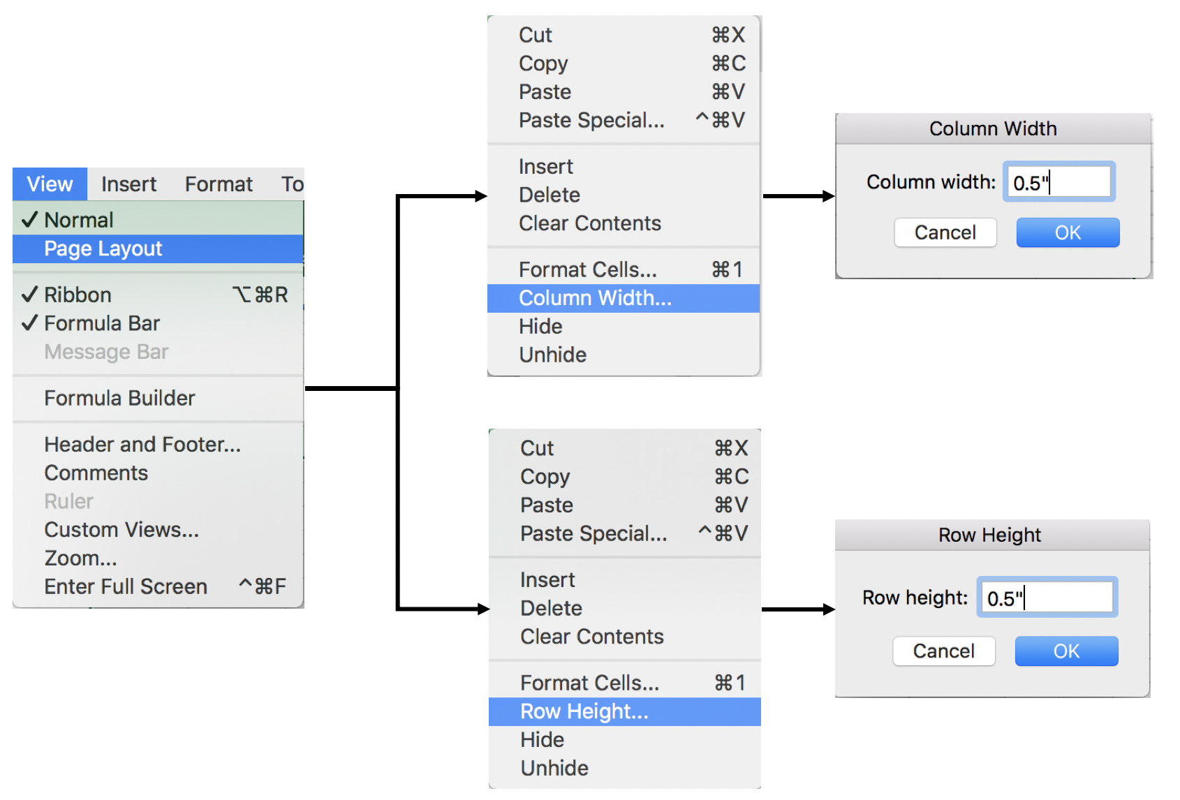
Step 1. Setting up the grid
In Excel, we want to create a 10 by 10 square grid. To do this, change your view from Normal to Page Layout. We are doing this because Excel has a unique way of measuring row and height size (they are not on the same scale under the Normal view). When you change to the Page Layout, the scales for the columns and rows are in inches. Set the size for the columns and rows to 0.5 inch. You should have a 10 by 10 grid with squared that have a height and length of 0.5 inch.
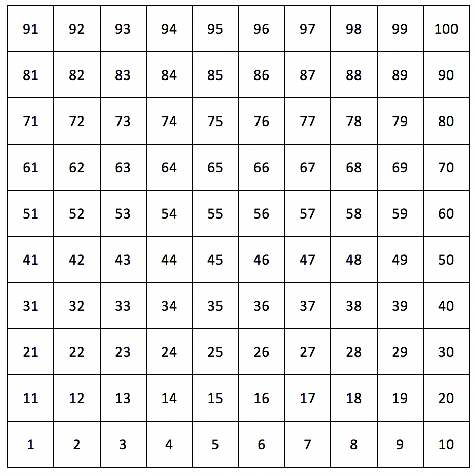
Step 2: Label the squares in the grid
Once the grid has been sized correctly, we will assign a value for each square in the grid. These values will correspond to the percentage point that you have in the cumulative values in Table 2. Start at the lower left with a cell value of 1 up to a cell value of 100 in the upper right of the grid.
Step 3: Apply conditional formatting for each cell in the grid
Once the cells have been assigned a value, we can use Excel’s conditional formatting tool to assign colors for each of expenditure components.
Select the cell that has the value “91.” (It doesn’t matter what cell you select, but we will use the upper-most left corner for simplicity; this is also cell D5).
Change the Select option to “Classic.” Then change the New Formatting Rule to “Use a formula to determine which cells to format.”

Insert the formula where you have the value is less than or equal to the total cumulative percentage (e.g., 100 percent).

The cells for the equations are specific to this example, but you can apply this towards an example of your own. (The Excel file that is based on this article can be downloaded here.)
Step 4: Change colors to match the different expenditure categories
Next, we will change the fill and font colors so that they will match. By having the font color the same as the fill color, the values in the cells will appear invisible, but still referenced using the conditional formatting rules we just created.

Step 5: Apply the conditional formatting to ALL the cells in the grid
After you change the colors for the font and fill, you will need to make sure that the conditional formatting rule is applied to the entire grid.

You should notice that all the cells in the grid are the same color. This is because the conditional formatting is first based on the total cumulative percentage, which is 100. Therefore, all the values in the cells should be the same color.

Step 6: Add a new conditional formatting rule for the next expenditure component
The next step is to apply another conditional formatting rule for the next highest cumulative percentage value, which would be Government Public Health Access, which is 89 percent.

We repeat the process for each expenditure component. When we are done, we should have four conditional formatting rules for each expenditure component.

All the formulas for the conditional formatting are listed below:

Step 7: Repeat this process for the other decades
Once we complete these conditional formatting for the other decades, we can present these waffle charts together.
Final waffle chart
The following waffle chart incorporated the health expenditures for each decade starting from 1965 to 2015. The border color was changed to white and the label used the Century Gothic font. Inside each waffle is the percentage of Investment associated with each decade. You can download this exercise’s Excel file here.

Based on the waffle charts, we can see that Investments (spending for noncommercial biomedical research and expenditures by health care establishments on structures and equipment) has decreased over time. Conversely, expenditures for Personal Health Care, Administration, and Health Activities have increased.
CONCLUSIONS
Using waffle charts is a better alternative to pie charts because we can discern the exact value of the parts that make up the whole. In this case, we can easily visualize the decrease in Investments when it comes to health expenditure spending in the US for each decade between 1965 to 2015.
You can re-create these findings using the Excel file located here.
REFERENCES
I used the following references to assist with the development of this article. They have been incredibly helpful in learning the methods and better understanding how to leverage the power of using waffle charts.
[1] Tufte ER. The Visual Display of Quantitative Information. 2001. Graphic Press. Cheshire. CT.
Everyday Office’s YouTube video
https://www.youtube.com/watch?v=HZe5SzgxlsQ
Michael Sandberg’s Data Visualization Blog
https://datavizblog.com/2014/09/09/dataviz-squaring-the-pie-chart-waffle-chart/
Robert Kosara’s Eagereyes Blog
https://eagereyes.org/techniques/pie-charts
Sumit Bansal’s Trump Excel: The Smart Way Blog
https://trumpexcel.com/waffle-chart-excel/
Jonathan Schwabish’s PolicyViz Blog provides another method to creating waffle charts using data validation
https://policyviz.com/2018/04/26/interactive-waffle-charts-in-excel/