
BACKGROUND
In time series analysis, we are interested on the impact of some exposure over a time period. Exposure can be coded as event==1. If this is time-varying, then the event can occur at any time across a time period. Time series analysis requires us to identify the time when the event first occurred. In most cases this is also considered the post period. In this example, we will label the exposure of interest as event.
Longitudinal data can come in either a wide or long format. However, it is easier to perform longitudinal data analysis in the long format. This assumes that you declare either the xtset or tsset as a panel or time-series data set, respectively.
MOTIVATING EXAMPLE
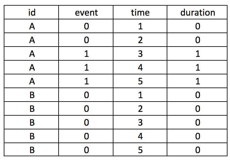
Let’s assume that we have two subjects (A and B), who can experience an event at any time between some time variable 1 and 5, time(1:5). This is a longitudinal data set in the long format with id as the unique subject-level identifier, the exposure variable of interest event as the exposure, and time as an arbitrary time variable ranging from 1 to 5. The event for subject A occurs at time==3.

Suppose you want to create a variable that counts the number of times the subject has the event. We will call this variable duration.

The following Stata code will generate the duration variable.
by id (time), sort: gen byte duration = sum(event==1)
Sorting by the id and then time will nest the time sequence for each id. The sum() will add all event that is coded as 1.
It’s critical that you put time in parentheses (); otherwise, you can generate incorrect values. For instance, if you make the mistake of typing the Stata code as follows, you will generate a dataset which doesn’t provide the cumulative duration of having the event. Notice how the duration variable only has 1 instead of 1, 2, and 3.
by id time, sort: gen byte duration = sum(event==1)
Similarly, if you use the following code, you will generate the incorrect values. The sum(event)==1 syntax should be sum(event==1). However, this will “flag” the time when the event first occurred, which may be useful in some cases.
by id (time), sort: gen byte duration = sum(event)==1

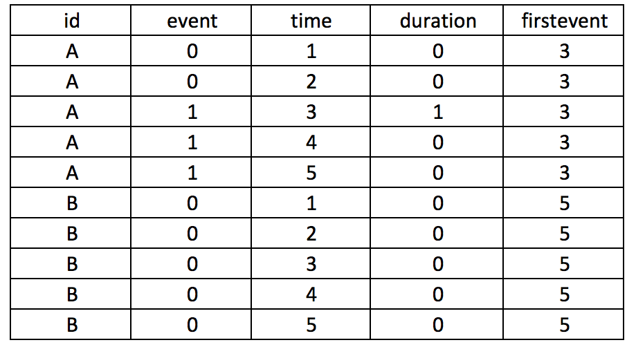
Let’s take our example further and generate a variable column that takes into consideration the period before the subject experiences an event. Suppose subject A experiences an event at time==3, but we want to center this as 0 and previous months as -1, -2, and so on. We need to first identify the time when the event occurs and populate that as a new variable, which we will call firstevent. We can use the following State code to generate firstevent based on the condition that the event==1 and the variable it occurs is time==3.
egen firstevent = min(cond(event == 1, time, .)), by(id)

There will be missing values since not all subjects experience the event. To populate the missing values for the subjects with no events (event==0), we need to replace firstevent by identifying the max time of the entire study period using the summary command. Once we have the max time of the study period, we add 1 to this and replace the missing values from the firstevent variable.
replace firstevent = max(time) if firstevent == .
summ time
global maxtime = r(max)

replace firstevent = $maxtime + 1 if firstevent == .
We can subtract the time from the first event to generate a new variable (its) that will capture the negative time before the event occurs and the positive time after the event occurs, centered on when event==1.
by id (time), sort: gen byte its = _n – firstevent

The new variable its is short for interrupted time series analysis. An investigator can use the its variable to plan any interrupted times series analysis without having to go through the ordeal of generating this variable using other software.
Here is a summary of the entire Stata code, which you can also find on my Github page:
***** Declare XTSET panel dataset.
* Variable list: id event time
* id        =   subject identifier
* event     =   exposure of interest
* time      =   time interval

**** Create the duration variable to capture time after event.
by id (time), sort: gen byte duration = sum(event==1)

**** Create a variable for the time before the event.
egen firstevent = min(cond(event == 1, time, .)), by(id)

**** Identify the maxtime.
summ time
global maxtime = r(max)

**** Replace missing data with the maxtime + 1.
replace firstevent = $maxtime + 1 if firstevent == .

**** Create its to capture time before and after event.
by id (time), sort: gen byte its = _n - firstevent
ACKNOWLEDGEMENTS
I used several online references to develop this tutorial for Stata. Nicholas J. Cox has some excellent tutorials that was influential in developing this piece.
Cox N. First and last occurrences in panel data. From https://www.stata.com/support/faqs/data-management/first-and-last-occurrences/
The Statlist forum was also helpful; in particular, the following discussion threads.
https://www.stata.com/statalist/archive/2010-12/msg00193.html
https://www.stata.com/statalist/archive/2012-09/msg00286.html
The UCLA Institute for Digital Research and Education has a tutorial on using _N and _n to count in Stata.
Counting from _N to _N. UCLA: Statistical Consulting Group. From https://stats.idre.ucla.edu/stata/seminars/notes/counting-from-_n-to-_n/