Excel programming

Using Excel VBA macros to conduct one-way sensitivity analyses and tornado diagram

INTRODUCTION

In pharmacoeconomic analysis, we oftentimes incorporate data from external sources to inform the parameters of our economic models. It’s not uncommon for us to have some degree of uncertainty surrounding the values of our parameters. The size and influence of each uncertainty may influence our conclusions, which can significantly change based on a single parameter. For instance, if a new drug (Drug A) entering the market had an incremental cost-effectiveness ratio (ICER) that was greater than the stakeholder’s willingness-to-pay (WTP) threshold when compared to standard of care (Drug B), lowering Drug A’s price may move the ICER to below the WTP threshold (Figure 1). This could change the conclusion of the study from “Drug A is not cost effective compared to Drug B,” to “Drug A is cost effective compared to Drug B.” Of course, this depends on where the WTP threshold is located on the cost-effectiveness plane, but it highlights the importance of understanding the influence of a single parameter to a pharmacoeconomic model’s conclusion. This type of analysis to understand the influence of a single parameter on the model’s conclusion can be illustrated using a one-way sensitivity analysis.

Figure 1. Example of the incremental cost-effectiveness ratio (ICER) changing due to a change in the price of Drug A.

Multiple one-way sensitivity analyses can be performed and arranged in a way to visualize the parameters with the greatest influence on the study’s outcome using a tornado diagram. The tornado diagram arranges the impact of each one-way sensitivity analyses from largest (top) to smallest (bottom) on the chart (Figure 2).

Figure 2. Example tornado diagram.

You can perform multiple one-way sensitivity analysis and arrange them in a tornado diagram using Excel’s Visual Basic Application (VBA) macros. In this tutorial, you’ll be able to create a series of VBA macros to conduct one-way sensitivity analyses and visualize these as a tornado diagram.


MOTIVATING EXAMPLE

We will use a hypothetical decision tree model to perform a series of one-way sensitivity analyses. You can download the Excel file and high resolution images for this tutorial from the GitHub repository for Decision Tree Tutorials here. The example decision tree and its parameters are illustrated in Figure 3.

Figure 3. Decision tree and relevant parameters.

The base-case ICER comparing Drug A to Drug B is $5875 per one additional Cure achieved (Figure 4). The ICER is located in the Northeast quadrant.

Figure 4. Results from the decision tree and cost-effectiveness plane.

We will create a macro that will replace the Base-case value with the LL and UL values (lower limit and upper limit, respectively) for every parameter and re-calculate the ICER each time.

Here is what the final one-way sensitivity analysis table will look like after the macros are run (Figure 5). Notice how the Number column is not in ascending order. That’s because this is ordered by the Spread column, which is the absolute difference between the UL_ICER and LL_ICER. We sort by the Spread because it allows for the tornado diagram to place the parameter with the greatest influence on the base-case ICER at the top and the parameter with the least influence at the bottom.

Figure 5. Results from the one-way sensitivity analysis.

We will create three macros. The first macro will sort the Number column in ascending order. This helps with the one-way sensitivity analysis calculations. The second macro will perform the one-way sensitivity analyses by replacing the Value with the LL or UL values. The last macro will sort the Spread in descending order for the tornado diagram.

Note: In this tutorial, the tornado diagram is already generated and mapped to the data on the one-way sensitivity analysis table. I wrote a tutorial on how to create a tornado diagram, which can be accessed here.

To create and edit macros, you will need to make sure that the Developer tab is available on the ribbon panel (Figure 6).

Figure 6. Developer tab on Excel’s ribbon panel.

In Excel, go to the File > Options. In the Options window, select Customize Ribbon and check the box next to Developer in the Main Tabs column (Figure 7).

Figure 7. Enabling the Develop tab in the Options window.

Once the Develop tab is enabled, we can begin to examine the macros. To open the VBA editor, go to the Develop tab and click on Macros as seen in Figure 8. There are several macros that we can see under the Macro window. Select the oneway_order macro and click on Edit. This will open the VBA editor where we can examine the macro.

Figure 8. Open the VBA editor.

The VBA editor has several important features.

In the left panel are the various macros and their location. The right panel contains the VBA code for the macro. The macro controls allow you run (“Play”), pause, or stop the macro.

Figure 9. VBA editor interface.

Note: Normally, we save our Excel file using the *.xlsx extension. However, when you have an Excel macro, you need to save the file as an *.xlsm extension. This will allow you to save your macros and enable them later.

VBA Macro 1 – Sorting the one-way sensitivity analysis table

Let’s examine the first macro: oneway_order

The VBA code first selects the sheet, which is labeled as OWSA model. Within the sheet, it selects the area defined by AM7:AV15 which is the one-way sensitivity analysis table in the Excel spreadsheet. The next part of the code orders the one-way sensitivity analysis table in ascending order based on the values in the Number column which is defined as AM8:AM15.

Note: Since this is on the same worksheet, we can leave the label of the active sheet as OWSA model. But if you were using different worksheets, you need to make sure to change the active sheet’s name.

The second part of the code tells the VBA macro to sort according to columns and that the first row contains the headers or column labels.

Figure 10. VBA Macro 1 – sort by ascending order the one-way sensitivity analysis table.

VBA Macro 2 – Re-calculate the ICERs with the lower and upper limits for each parameter

The second macro performs the one-way sensitivity analysis, and it is labelled as oneway_macro. Let’s take a close look at the VBA code for this macro. Notice how there is a low and high component in this macro. This is due to the LL and UL on the parameters table in the decision tree model. The oneway_macro will replace the base-case values with the value from the LL and UL columns in the decision tree model. This will need to be repeated for each parameter. In this decision tree model, there are 8 parameters that we will perform the one-way sensitivity analyses on. For the VBA macro, we will call these 0 to 7.

Figure 11 provides a close inspection of the macro and its elements in relation to the decision tree model in Excel. Notice that this is a loop function. The loop will start at 0 and end at 7 iterations, which is a total of 8 iterations, the same number of parameters in the decision tree. In the VBA macro, this is initiated with For low = 0 to 7 and then repeats with Next low until it reaches 8 iterations.

By changing these parameters with the LL and UL values, the ICER will be re-calculated. Once recalculated, we can update the one-way sensitivity analysis table with the new ICER value. In the VBA macro the re-calculated ICER is in cell AI7, and its value is imputed into the one-way sensitivity analysis table starting at cell AT8.

One the VBA macro completes, all 8 parameters will have undergone the one-way sensitivity analyses, and the re-calculated ICERs would be imputed into the one-way sensitivity analysis table; the LL_ICER and UL_ICER columns will contain the re-calculated ICERs for the LL and UL values from the parameters table.

Figure 11. VBA macro to perform series of one-way sensitivity analyses.

VBA Macro 3 – Re-sort the one-way sensitivity analysis table using the “Spread” in descending order

Once the ICERs have been re-calculated using the LL and UL from the parameters table, we can estimate their influence by calculating the absolute difference between the UL_ICER and LL_ICER. We want the absolute difference because we’re interested in visualizing the difference with the low and high values from each parameter.

Here is what VBA Macro 3 looks like:

This is very similar to the VBA Macro 1, which orders the one-way sensitivity analysis table based on the Number column. The only difference is that instead of using the Number column, VBA Macro 3 will sort in descending order the one-way sensitivity analysis using the Spread column, which contains the absolute difference between UL_ICER and LL_ICER.

Let’s take a look at the VBA macro closely (Figure 12).

Figure 12. VBA Macro 3 – re-order the one-way sensitivity analysis table by “Spread.”

The macro first selects the one-way sensitivity analysis table (AM7:AV15). It then selects the Spread column to sort in descending order (AM8:AM15). Once sorted, the macro will end.

Note: You may notice that the Order:=xlAscending option may sound counter-intuitive since we are sorting by descending order. The reason why the option has this in xlAscending order is because the tornado diagram uses a reverse axis on the Format Axis option (see Figure 13).

Figure 13. Format axis option to have the categories in reverse order.

Assigning macros

Once the one-way sensitivity analysis table is completed, we can assign these macros to buttons on the worksheet.

We can create buttons using the Shapes function in Excel. Right-click on the shape and select Assign macro. Create three of these. Figure 14 illustrates the steps to assign macros to each button.

Figure 14. Assigning macros to buttons in Excel.

We will assign oneway_order macro to the first button (Figure 15).

Figure 15. VBA Marco 1 assigned to the “Step 1” button.

We do the same thing for VBA Macro 2 (Figure 16).

Figure 16. VBA Macro 2 assigned to the “Step 2” button.

Lastly, we assign the final VBA macro to the “Step 3” button (Figure 17).

Figure 17. VBA Macro 3 assigned to the “Step 3” button.

Final steps

One all the buttons have been assigned to a VBA macro, we can click on each one in order to repeat the steps of re-calculating the ICER and updating the one-way sensitivity analysis table.

We can also see the changes to the tornado diagram (Figure 18).

Figure 18. Final tornado diagram.

At this stage of the tutorial, it’s good practice to inspect your entire Excel file to ensure that no data was accidentally lost or erased during the creating of the macros. Sometimes, if we select the wrong cells, we can overwrite our data. It’s good practice to save different versions of the Excel file so that you can return to your previous work in case something goes wrong.


Conclusions

Excel provides a power tool to generate VBA macros to perform functions iteratively. We leveraged this tool to perform a series of one-way sensitivity analyses which we then used to create a tornado diagram. Since this tutorial used a single worksheet, the process is much easier to code and diagnose. However, as we expand and create more worksheets in our Excel file, we need to be careful to select the proper sheets when using these VBA macros.


Acknowledgements

I used templates of previous one-way sensitivity analyses to build these VBA macros in this tutorial. Admittedly, it has been years since I first began doing this in Excel, and I don’t recall the sources. However, I wanted to acknowledge them as they deserve all the credit for helping me understand and apply these tools to building pharmacoeconomic models. If I find out the sources of these macros, I will post them here. I do know that my courses at the University of Washington was a source for some of the VBA macros for constructing pharmacoeconomic models, and I wanted to acknowledge their work and materials.


References

You can download the Excel file(s) from the GitHub Repository on Decision Tree Tutorials (link).


Disclaimers

This is a work in progress, therefore, there may be updates in the future.

This is for educational purposes only.

Constructing a Markov model for cost-effectiveness analysis using Excel: A tutorial

I wrote a tutorial on how to construct a Markov model using Excel, which is available on my RPubs site (link). This was meant to complement a workshop that I am preparing for trainees interested in pharmacoeconomics.

The Markov model is a versatile mathematical model that allows researchers to simulate a chronic disease for many years. It is unique due to its features such as disease states which can contain the costs and benefits associated with them.

I posted files associated with this tutorial on my GitHub Markov Model Tutorial respository (link). These include some readings to provide sufficient background and the Excel file with the Markov model example. To properly download these files, make sure to go to the “Raw” file and right clich on the “Raw” option then “Save link as” onto your computer. There is a detailed explanation on the RPubs tutorial.

This is a work in progress, so expect some updates in the future.

Communicating data effectively with data visualizations - Part 10 (Heat Maps)

BACKGROUND

A heat map is a data visualization tool that uses positioning and coloring to identify clusters and correlations in multivariable analysis. The most common type of heat map is a 2 x 2 matrix, where two variables are examined using the rows and columns (R x C) positions on a matrix. A heat map matrix helps us identify any patterns or similarities across the different dimensions. In a heat map, color is critical in denoting degrees of change. (Please see refer to the past blog on colors.)

For example, we can see the changes in opioid overdose rates across time for each state (Figure 1). As the rates increase, the cells are darker (indicated by the legend). All the states experience an increase in opioid overdose deaths, but State 1 is experiencing it faster than States 2 and 3.

In this tutorial, we will perform two methods to create heat maps. The first method will use the built in Excel conditional formatting rules and the second method will use VBA macros.

Figure 1. Heat map matrix.

Figure 1 - heatmap matrix.png

MOTIVATING EXAMPLE

We will continue to use the state-level drug overdose mortality data from the CDC.

https://www.cdc.gov/drugoverdose/data/statedeaths.html

Mortality rate is presented as the number of deaths per 100,000 population.

In this tutorial, we will develop a heat map using opioid overdose mortality from 2013 to 2016.

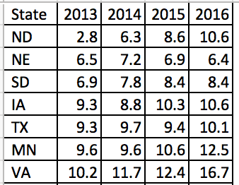
The data setup in Excel has State indicators as the rows and time indicators as the columns. We are visualizing the change in opioid overdose mortality from 2013 to 2016 for each state. Figure 2 illustrates the data structure for the first seven states.


Figure 2. Data structure for the first seven states.  

Figure 2 - Data structure.png


METHOD 1: CONDITIONAL FORMATTING RULES

Excel has a convenient tool that allow us to use conditional formatting to shade our heat map matrix.

Step 1: First highlight all the data.


Step 2: In the Excel Ribbon, select Conditional formatting and then New.

Figure 3 - conditional formatting.png

Step 3: Select “Format all cells based on their values” and change the Format Style to “3-Color scale.” Change the color to the different shades you are interested in using. (In this example, we used a blue base with varying degrees of shading.) Select percentile and then click “Ok.” The percentile will use the Median for each column to distinguish the middle category for the rates of opioid overdose mortality for each state.

Figure 4 - 3-color scale.png

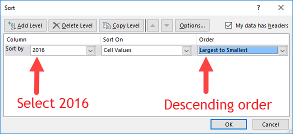
Step 4: Visually inspect the results. If there are no apparent pattern in the heat map, we will need to sort the rate of opioid overdose mortality for 2016 in descending order.

Figure 4 - Descending order.png

The heat map should look like the following:

 
Figure 6 - heat map example 1.png
 

There is a pattern emerging in regards to the rate of opioid overdose mortality across the different states. West Virginia has the highest opioid overdose mortality rate in 2016, but they also appear to have the highest from 2013 to 2015. The dark cell in 2016 indicates that West Virginia has exceeded the 50 deaths per 1000 population incidence rate. Other states also have high rates of opioid overdose mortality across 2013 to 2016, which continued to increase. The 2013 column is clearly lighter indicating that the opioid overdose mortality has increased over time up to the available data in 2016.


Step 5: We can improve this heat map by removing the numbers, which can be distracting. We need to select all the data and format the cells. Select only the numeric data and then format the number. Use the “Custom” category and enter the following: "";"";"";"". This will change the number values so that it doesn’t show in the cells.

Figure 7 - change the number format.png

Step 6: Change the column width and row height so that you have a nice square-like matrix for the final result. We used a column width of 5 and a row height of 30. (Only the first fifteen states are shown.)

The heat map can be used to quickly identify states with the highest opioid overdose mortality and the trends across time. The states with the highest rates of opioid overdose mortality are clustered at the top while the states with the lowest rates are clustered at the bottom.

We could also arrange this into regions of the US to further stratify the results (not shown).


METHOD 2: USING VBA MACROS FOR CONDITIONAL FORMATTING OF MORE THAN 3 CATEGORIES

Excel only allows us to choose up to 3-Color scales. If we wanted to use more than 3 color categories, we will need to use VBA macros.

But before we do, we need to think about the colors for the scales. Since we have more than 3 categories, we will need to figure out how to divide the colors.


COLOR CODES

We will need to determine the base color for our heat map. In this example, we will use a blue base-color and change the shading using the RGB color values. RGB colors are based on a system using a combination of three base colors (red, green, and blue) that can be used to change the intensity of the color from a range between 0 and 250. An example of an RGC color table can be found in the following site.

For this example, we used the following RGB color values where dark-navy denotes high rates of opioid overdose mortality (50 or more per 1000 population). However, you can change the values of these colors however you like.

Figure color codes.png

We will continue to use the blue color base and change the gradient using the RGB values.


VISUAL BASIC FOR APPLICATION (VBA) MACRO

The VBA macro comes from the site Excel For Beginners and written by Kristoff deCunha. We used the VBA code on the site, but modified it for this tutorial.

The VBA code is written in a way where any changes in the values will automatically update the color of the cell. Additionally, the code also sorts the 2016 opioid overdose mortality rate in descending order, adds thin-white continuous borders around the cells, and changes the font to Times New Roman.

Here are the VBA macros used for Method 2.


Macro 1 changes the font to Times New Roman.

‘Macro1
Sub ChangeFont()

Dim rng As Range
Set rng = Range("J1:N52")

With rng.Font
    .Name = "Times New Roman"
    .Size = 12
    .Strikethrough = False
    .Superscript = False
    .Subscript = False
    .OutlineFont = False
    .Shadow = False
    .Underline = xlUnderlineStyleNone
    .ThemeColor = xlThemeColorLight1
    .TintAndShade = 0
    .ThemeFont = xlThemeFontNone
End With

End Sub


Macro 2 changes the cell shading to the 6-Color scale (blue-base)

‘Macro2
Sub ChangeCellColor()


Dim rng As Range
Dim oCell As Range

Set rng = Range("K2:N52")

For Each oCell In rng
        Select Case oCell.Value
                 Case 50 To 100
                     oCell.Interior.Color = RGB(37, 54, 97)
                     oCell.Font.Bold = True
                     oCell.Font.Name = "Times New Roman"
                     oCell.HorizontalAlignment = xlCenter
                 Case 40 To 49.999
                     oCell.Interior.Color = RGB(56, 83, 145)
                     oCell.Font.Bold = True
                     oCell.Font.Name = "Times New Roman"
                     oCell.HorizontalAlignment = xlCenter
                 Case 30 To 39.999
                     oCell.Interior.Color = RGB(147, 168, 215)
                     oCell.Font.Bold = True
                     oCell.Font.Name = "Times New Roman"
                     oCell.HorizontalAlignment = xlCenter
                 Case 20 To 29.999
                     oCell.Interior.Color = RGB(183, 198, 228)
                     oCell.Font.Bold = True
                     oCell.Font.Name = "Times New Roman"
                     oCell.HorizontalAlignment = xlCenter
                 Case 10 To 19.999
                     oCell.Interior.Color = RGB(218, 225, 240)
                     oCell.Font.Bold = True
                     oCell.Font.Name = "Times New Roman"
                     oCell.HorizontalAlignment = xlCenter
                 Case 0 To 9.999
                     oCell.Interior.Color = RGB(230, 237, 253)
                     oCell.Font.Bold = True
                     oCell.Font.Name = "Times New Roman"
                     oCell.HorizontalAlignment = xlCenter
                  Case Else
                     oCell.Interior.ColorIndex = xlNone
         End Select
    Next oCell
    
End Sub


Macro 3 sorts the 2016 opioid overdose mortality rates in descending order.

‘Macro3
Sub SortColumn()

Dim DataRange As Range
Dim keyRange As Range
Set DataRange = Range("J1:N52")
Set keyRange = Range("N1")
DataRange.Sort Key1:=keyRange, Order1:=xlDescending

End Sub


Macro 4 hides the font from the heat map.

‘Macro4
Sub HideFont()
    
Dim rng As Range
Dim oCell As Range

Set rng = Range("K2:N52")

    For Each oCell In rng
        oCell.Font.Color = oCell.Interior.Color
    Next oCell
    
End Sub


Macro 5 creates thick white borders for each cell in the table.

‘Macro5
Sub WhiteOutlineCells()

    Dim rng As Range

    Set rng = Range("J1:N52")

    With rng.Borders
        .LineStyle = xlContinuous
        .Color = vbWhite
        .Weight = xlThick
    End With
    
End Sub

INSERTING DATA AND RUNNING MACRO

The five macros are assigned to a button in the Excel Macro-Enabled Workbook. Pressing the button will perform the task of creating a 6-Color scale heat map. Download the Excel Macro-Enabled Workbook here. This file will have the raw data and the macro-enabled worksheet for you to create a heat map.

Step 1: Copy the raw data from the “combined” worksheet.

Figure 9 - Copy Data.png

Step 2: Paste it in the worksheet “heatmap_2” starting on cell "J1".

Figure 10 - Copy onto J1.png

Step 3: Then press the “PressStart” button to run the macros. Your final heat map should look like the following:

Compare the heat map from Method 1 (3-Color scale) to the one generated by Method 2 (6-Color scale). The heat map with the 6-Color scale has a lighter pattern compared to the 3-Color scale heat map. The differences are dramatic. Depending on the granularity of the heat map you want, either one of these color scales would be fine. However, Method 2 requires some VBA coding.

* Not all states shown.


Conclusions

Heat maps allow us to observe patterns in the data. In our example, we notice that West Virginia has a high rate of opioid overdose mortality indicated by the clustering of dark cells from 2013 to 2016. Other states had similar patterns as West Virginia. Using heat maps provides a quick and easy interpretation of the changes in opioid overdose mortality across time and the states that are clustered together that have high rates of opioid overdose mortality.


REFERENCES

I used the following websites to help develop this tutorial.

Conditional formatting with more than 3 categories:
https://sites.google.com/site/excelforbeginners/Home/vba-codes/conditional-formatting-more-than-3-criterias
 
Changing the RGB color codes:
https://analysistabs.com/excel-vba/change-background-color-of-cell-range/
https://www.w3schools.com/colors/colors_rgb.asp

Excel color palette library:
http://dmcritchie.mvps.org/excel/colors.htm

Excellent site for VBA coding:
https://www.excel-easy.com/vba.html


Excel macro to convert cell values in a pivot table from COUNT to SUM

Background

I was preparing a report for the Veterans Health Administration and I ran into an inconvenience where I had to convert the values in a pivot table from the default COUNT to SUM. Normally, this would not be an onerous process. However, there were several columns that I wanted to convert, which would take an enormous amount of work to perform. Fortunately, I ran into Doctor Moxie's blog, which providers tips and tricks to using Excel efficiently. You can find the blog here.

Doctor Moxie created a Visual Basic Macro that conveniently converts all the data in the pivot table from the default COUNT to SUM.


Motivating Example

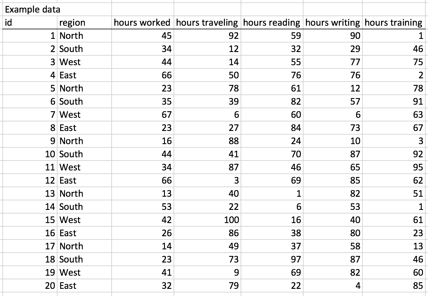
To illustrate the solution, I used the following example dataset, which was generated using the following function:

=RANDBETWEEN(0, 100)

This will generate a value between 1 and 100 for each cell.

Screen Shot 2018-02-01 at 3.38.09 PM.png

I used the pivot table to see see the number of hours per region. From the pivot table, the values were reported as COUNT per region instead of SUM per region.

Screen Shot 2018-02-01 at 3.40.47 PM.png

I could go through each column and change the values from COUNT to SUM, but this would be inconvenient if there were over 100 columns.

Doctor Moxie developed an inventive solution to address this problem using a macro, which you can get from his/her website.

Using the macro converted the values from COUNT to SUM.

Screen Shot 2018-02-01 at 3.45.35 PM.png

The macro nicely converts all the cells and makes the analysis easier to perform. This saved me hours of work and I recommend you keep this macro in your Excel arsenal.


Acknowledgements

Doctor Moxie is credited with developing the macro and his/her website (ExcelPivots) can be found here.