Cobb-Douglas production function and costs minimization problem

Update 2: This article was updated on 12 August 2023 when Dimanjan Dahal (Twitter account) identified a better way to present the Lagrangian functions. I updated this to better reflect the minimization problem and set the partial derivative solution to 0. Thank you, Dimanhan.

Update 1: This article was updated on 11 October 2021 when an anonymous reader identified an error with the example used at the end. The error was the negative value generated for the output elasticity of capital. In the previous example, I used R to generate a set of random numbers that were used in a regression model. The beta coefficient generated a negative value which was used in the linear form of the Cobb-Douglass equation. Since the output of elasticity should be between the values of 0 and 1, this negative coefficient should not be possible. Hence, I’ve updated the data frame used in the example to avoid this issue. Appreciation goes out to the anonymous reader who identified this error.

INTRODUCTION

The Cobb-Douglas (CD) production function is an economic production function with two or more variables (inputs) that describes the output of a firm. Typical inputs include labor (L) and capital (K). It is similarly used to describe utility maximization through the following function [U(x)]. However, in this example, we will learn how to answer a minimization problem subject to (s.t.) the CD production function as a constraint.

The functional form of the CD production function:

where the output Y is a function of labor (L) and capital (K), A is the total factor productivity and is otherwise a constant, L denotes labor, K denotes capital, alpha represents the output elasticity of labor, beta represents the output elasticity of capital, and (alpha + beta = 1) represents the constant returns to scale (CRS). The partial derivative of the CD function with respect to (w.r.t) labor (L) is:

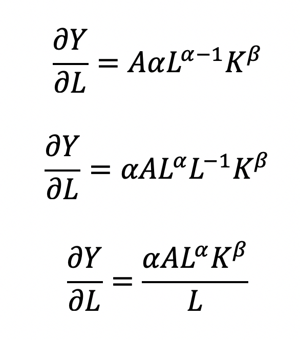
Recall that quantity produced is based on the labor and capital; therefore, we can solve for alpha:

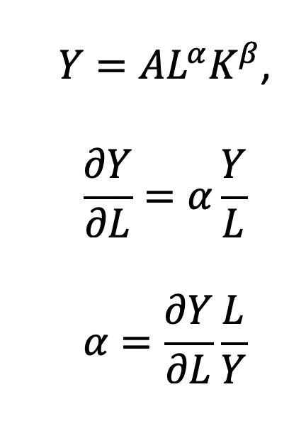
This will yield the marginal product of labor (L). If alpha = 2, then a 10% increase in labor (L) will result in a 20% increase in output (Y).

The partial derivative of the CD function with respect to (w.r.t) labor (K) is:

This will yield the marginal product of capital (K).

The CD production function can be converted to a linear model by taking the logarithm of both sides of the equation:

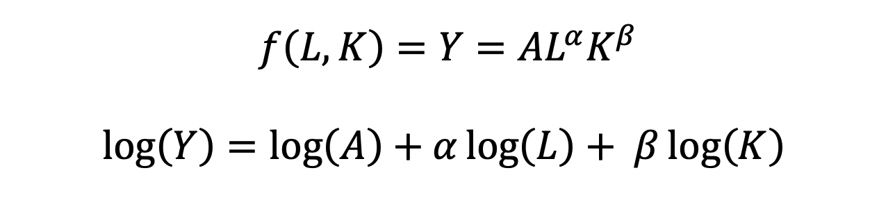
This will allow for OLS regression methods, which is commonly used in economics to understand the association between inputs (L and K) on production (Y).

However, what happens when we are interested in the marginal cost with respect to (w.r.t.) production (Y)? This becomes a constraint (cost) minimization problem where the firm can control how much L and K they will use. In other words, we want to minimize the cost subject to (s.t.) the output

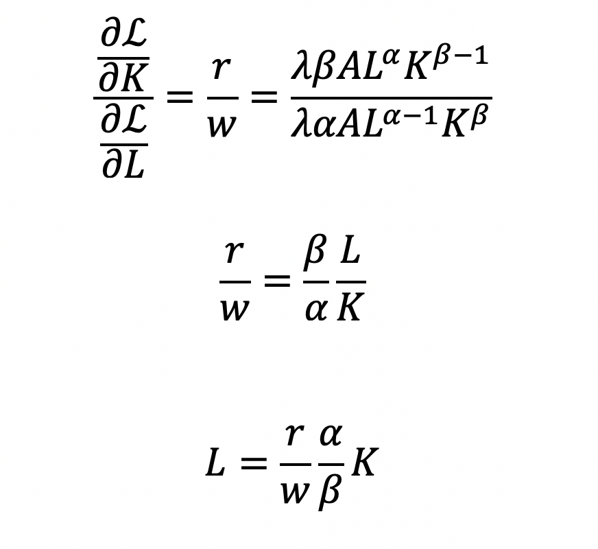
Cost becomes a function of wage (w), the amount of labor (L), price of capital (r), and the amount of capital (K). To determine the optimal amount of inputs (L and K), we solve this minimization constraint using the Lagrange multiplier method:

View fullsize

Solve for L

Substitute L in the constraint term (CD production function) in order to solve for K

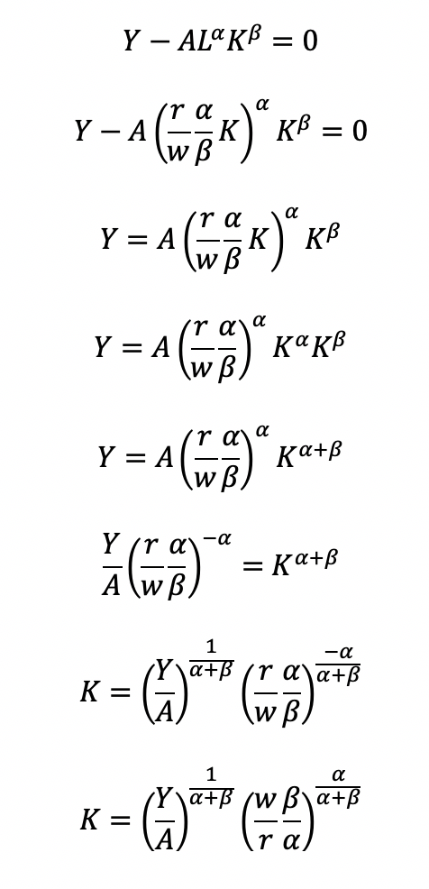
Now, we can completely solve for L (as a function of Y, A, w, and r) by substituting for K

Substitute L and K into the cost minimization problem

Simplify

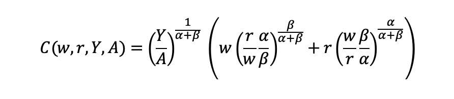
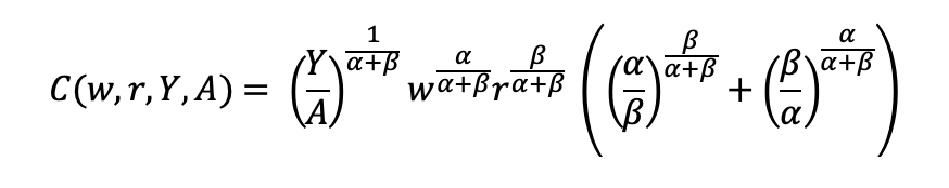
Final cost function

Let’s see how we can use the results from a regression model to give us information about the total costs w.r.t. to the quantity produced.

Recall the linear form of the Cobb-Douglas production function:

I simulated some data where we have the capital, labor, and quantity produced in R.

## Use the following libraries:
library(jtools)
library(broom)
library(ggstance)
library(broom.mixed)

## Generate random data for the data frame (cddata)
set.seed(1234)

production <- sample(100:600, 30, replace=TRUE)

labor <- sample(50:350, 30, replace=TRUE)

capital <- sample(6000:7000, 30, replace=TRUE)

## Cost function parameters: wage and price constants
wage <- 35.00
price <- 30.00

## Set up the data frame (cddata):
cddata <- data.frame(production = production, labor = labor, capital = capital, wage = wage, price = price)

## Name rows using some timeline from 1988 to 2017 (30 years for 30 observations for each variable):
row.names(cddata) <- 1988:2017

Then I perform a regression model using OLS

## Setting up the model, where log(a) is eliminated due to it being the intercept.
cd.lm <- lm(formula = log(production) ~ log(labor) + log(capital), data = cddata)

summary(cd.lm)

Residuals:
     Min       1Q   Median       3Q      Max 
-0.96586 -0.25176  0.06148  0.37513  0.67433 

Coefficients:
             Estimate Std. Error t value Pr(>|t|)
(Intercept)   4.44637   17.41733   0.255    0.800
log(labor)    0.14373    0.23595   0.609    0.548
log(capital)  0.05581    2.00672   0.028    0.978

Residual standard error: 0.5065 on 27 degrees of freedom
Multiple R-squared:  0.01414,   Adjusted R-squared:  -0.05888 
F-statistic: 0.1937 on 2 and 27 DF,  p-value: 0.8251

After running the model, I stored the coefficients for use later in the production function.

## Store the coefficients
coeff <- coef(cd.lm)

## Assign the values to the production function parameters where Y = AL^(alpha)K^(beta)
intercept <- coeff[1]
alpha <- coeff[2]
beta <- coeff[3]

From the parameters, we can get A (intercept), alpha (log(labor)), and beta (log(capital)).

This will give us the quantity produced (Y) for given data on labor (L) and capital (K).

We can get the total costs (C) based on the quantity produced (Y) using the cost function:

I set up my R code so that I have the intercept, alpha, beta, labor, wage, and price of the capital set up. I estimated each part of the cost function separately and then multiply the parts at the end.

## Cost
PartA <- (production / intercept)^(1 / alpha + beta)
PartB <- wage^(alpha / alpha + beta)
PartC <- price^(beta / alpha + beta)
PartD <- as.complex(alpha / beta )^(beta / alpha + beta) + as.complex(beta/ alpha)^(alpha / alpha + beta)

costs <- PartA * PartB * PartC * PartD

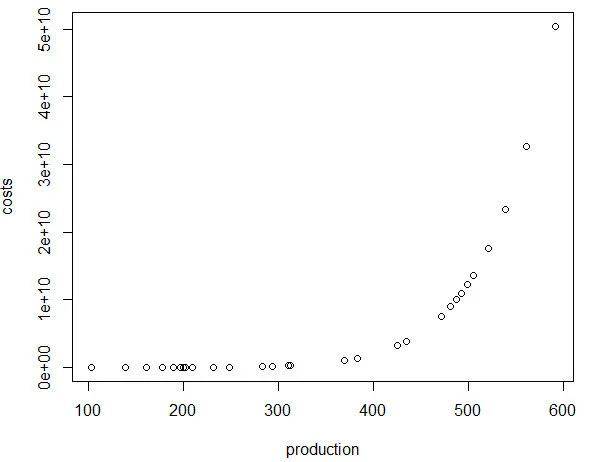
Note: R has a problem with performing complex operations with exponents that were defined using arrays or vectors. If you try to compute something like x^{alpha}, you will get an error where the value is “NaN.” I don’t have a complete understanding of the problem, but the solution is to make sure your root or base term is preceded by “as.complex(x)” to resolve the issue.

I plot the relationship between quantity produced and cost. In other words, this tells us the lowest costs needed to produce the quantities on the plot.

plot(production, costs)

CONCLUSIONS

Using the Cobb-Douglas production function and the cost minimization approach, we were able to find the optimal conditions for the cost function and plot the outcome relative to the quantity produced. As production increases, the minimum cost needed increases in a non-linear, exponential fashion, which makes sense given that Y (quantity produced) is in the numerator on the right-hand side of the cost function and positively related to the cost.

This was a fun exercise that made me think about the usefulness of the Cobb-Douglas production function, which I learned to optimize multiple times in my Economics courses. I was excited to find a pleasant utility for it using simulated data and will probably explore more exercises like this in the future.

REFERENCEs

I used a lot of resources to write this blog, which are provided below.

A site dedicated to the discussion of economics called EconomicsDiscussion.net was a great resource.

These papers were incredibly helpful in preparing the example in R:

• Lin CP. The application of Cobb-Douglas production cost functions to construction firms in Japan and Taiwan. Review of Pacific Basin Financial Markets and Policies Vol. 5, No. 1 (2002): 111–128.

• Larriviere JB, Sandler R. A student friendly illustration and project: empirical testing of the Cobb-Douglas production function using major league baseball. Journal of Economics and Economic Education Research, Volume 13, Number 3, 2012: 81-92

• Hu, ZH. Reliable Optimal Production Control with Cobb-Douglas Model. Reliable Computing. 1998; 4(1): 63-69.

I encountered some issues regarding complex numbers in R. Fortunately, I found some great resources about it.

• I found a great discussion about R’s calculation of exponents and “NaN” results and why complex numbers can mess up your math in R.

• Another good site (R Tutorial: An Introduction to Statistics) explaining complex numbers in R.

• John Myles White wrote a nice article about complex numbers in R.

Acknowledgements: I would like to thank the user who reached out to me about the coefficient errors for the output elasticity of capital. This helps me to learn my mistakes and correct them. Without the support and guidance from the community, I would not achieve my own goals of being a lifelong learner. Thank you.

Using Stata’s bysort command for panel data in time series analysis

BACKGROUND

Sorting information in panel data is crucial for time series analysis. For example, sorting by the time for time series analysis requires you to use the sort or bysort command to ensure that the panel is ordered correctly. However, when it comes to panel data where you may have to distinguish a patient located at two different sites or a patient with multiple events (e.g., deaths), it’s important to organize the data properly.

You can download the sample data and Stata code at the following links:

Data

Code

MOTIVATING EXAMPLE

In this example, we have a data set with time (months) in the column and patients in the rows (this is called a wide format data set). For each month, there are different numbers of observations. For instance, in Month 1, there were 5 observations. But in Month 7 there were only three.

The highlighted boxes indicate a patient was observed at two different sites. There are two ways to approach this: (1) remove the patient from Site B or (2) keep the patient by distinguishing it at each sight. Removing the patient will result in a loss of information for Site B, but keeping the patient complicates the panel data when we convert from wide to long format.

Converting this from wide to long format would result in the following panel data. Review each patient, in particular, the months of observations reported for the months. Notice that not all patients have observations for all the months (Months 1 to 7). Some patients have observations for scattered months (e.g., Patient 3). Of note is Patient 2 who has observations at Sites A and B. Since we opted to keep Patient 2 data for Sites A and B, we need to distinguish a method to ensure that the panel data is ordered correctly. Interestingly, Patient 8 has an observed event  (Death) three times at Months 5, 6, and 7. Since a patient should experience death only once, this may be a coding error and should be removed. Using the Stata sort and bysort command will allow us to fix this problem.

The bysort command has the following syntax:

bysort varlist1 (varlist2): stata_cmd

Stata orders the data according to varlist1 and varlist2, but the stata_cmd only acts upon the values in varlist1. This is a handy way to make sure that your ordering involves multiple variables, but Stata will only perform the command on the first set of variables.

REMOVE REPEATED DEATHS FROM PATIENT 8

First, we want to make sure we eliminate the repeated deaths from Patient 8. We can do this using the bysort command and summing the values of Death. Since Death == 1, we can sum up the total Deaths a patient experiences and drop those values that are greater than 1—because a patient can only die once.

***** Identify patients with repated death events. 
bysort id site (month death): gen byte repeat_deaths = sum(death==1)
drop if repeat_deaths > 1 

The alternative methods use the sort command:

* Alternative Method 1:
by id site (month death), sort: gen byte repeat_deaths = sum(death==1)
drop if repeat_deaths > 1

* Alternative Method 2:
sort id site (month death)
by id site (month death): gen byte repeat_deaths = sum(death ==1)
drop if repeat_deaths > 1

Now we have a data set without the unnecessary death values for Patient 8. Therefore, Patient 8 will not be counted in months 6 and 7 because they are no longer contributing to the denominator.

COUNT THE NUMBER OF DEATHS PER MONTH

Suppose we want to perform a single group time series analysis. We would want to sum up the number of deaths across the months. We can do this using the bysort command.

First, we have to think about how we want to count death. Since Death == 1, we want to add up the number of Death for each month. Initially, we were worried that Death would be counted two more times for Patient 8, but we solved this problem by removing these events from Patient 8.

The following command will yield the above results in a long format.

bysort month: egen byte total_deaths = total(death)

We use the egen command because we are using a more complex function. Detailers on when to use gen versus the egen commands are located at this site.

DETERMINING THE DENOMINATOR—COUNTING THE NUMBER OF PATIENTS CONTRIBUTION INFORMATION

Next, we want to determine that number of patient observations that are contributed to each month. To do this, we can use the bysort command again.

***** Determine the denominator -- using bysort and counter variable
gen counter = 1
bysort month: egen byte total_obs = total(counter)

This should yield the following results:

CHANGING FROM PATIENT-LEVEL DATA TO SINGLE-GROUP DATA

Currently, the data is set up using the patient-level. We want to change this to the single-group level or the aggregate monthly level. To do this, we have to eliminate the repeated month measurements for our total deaths (numerator) and total observations (denominator).

***** Drop duplicate months
bysort month: gen dup = cond(_N==1, 0, _n)
drop if dup > 1

We can visualize this by plotting two separated lines connected at the values for each month.

****** Plot the total number of deaths and total number of observations
graph twoway (connected total_deaths month, lcol(navy)) ///
             (connected total_obs month, lcol(cranberry) ytitle("Number") ///
	      xtitle("Months") ylab(, nogrid) graphregion(color(white)))

We can take this a step further and calculate the prevalence.

***** Estimate the prevalence (per 100 population) and plot
gen prev = (total_deaths / total_obs ) * 100	

graph twoway connected prev month, ytitle("Prevalence of Death" "per 100 population") ///
	     xtitle("Months") ylab(, nogrid) graphregion(color(white))

CONCLUSIONS

Using the bysort command can help us fix a variety of data issues with time series analysis. In this example, we have patient-level data that contained deaths for one patient and a patient who was observed at different sites. Using the bysort command to distinguish between sites allowed us to properly identify the patient as unique to the site. Additionally, we used the bysort to identify the patient with multiple deaths and eliminated these values from the aggregate monthly values. Then we finalized out single-group data set by summing the total deaths and observations per month and removing the duplicates.

You can download the Stata code from my Github site.

REFERENCES

I used the following references to write this blog.

Stata commands: bysort:

https://stats.idre.ucla.edu/stata/faq/can-i-do-by-and-sort-in-one-command/

Stata commands: gen versus egen:

https://stats.idre.ucla.edu/stata/seminars/notes/stata-class-notesmodifying-data/

Is my d20 killing me? – using the chi square test to determine if dice rolls are bias

BACKGROUND

Every Tuesdays, my friends and I enjoy playing role playing games (RPGs), especially table top RPGs such as Dungeons & Dragons (D&D). Every week, we get together and pull out our laptops, character sheets, and review our previous notes to return to the fictional fantasy worlds we created (or were created for us) and do battle, solve mysteries, and tell stories over some ciders (and Le Croix). This ritual is important because it allows us to disconnect from the real world and allow our imaginations to run wild. After every session, we think about the various actions that took place and review how things would have been different if the roll of a dice went a different way.

I first started playing D&D Second Edition when I was a kid after I was exposed to it at a comic book store (Golden Apple Comics in Los Angeles). I still remember the strange colorful dice rolling on a table top mat and people scratching away at paper using stats that I wasn’t familiar with. In high school, my friends and I would play different campaigns from the D&D and Forgotten Realms worlds, creating characters based on rule books using statistics and probabilities. The key ingredient with any adventure is having your fate determined by a single dice roll. The iconic dice in RPG is the d20 or the 20-sided dice. A d20 dice is usually used to determine whether you “hit” your opponent, use your skills to identify if a trap has been set or whether or not you can charm your way out of an unnecessary fight. Often times than not, there is the chance that a critical fail (a d20 roll of 1) can occur. When this happens, you fail to hit your opponent and trip over yourself during combat, miss the trap and activate it killing someone in your party, or pissing off the non-playable character (NPC) and having them attack you. Not only will something go wrong, it will go wrong spectacularly. So, it’s only natural that we look at the d20 that was rolled and ask, “Is my d20 killing me?”

Luckily, there is a statistical test that we can use to answer this common question.

CHI SQUARE TEST

The chi square test is one of the most common statistical tests performed in sciences. In its simplest form, the chi square test is used to detect whether the observed frequencies are different from the expected frequencies across different categories. For example, in a 6-sided dice, the probability that the number 6 will land is 16.7% or 1/6. This is true for every value of the 6-sided dice if it was unbiased.

But what if the dice was biased? Suppose we roll the 6-sided dice 100 times and we get the following results:

Visually, we can see that there is some bias with this 6-sided dice. We don’t know what the bias is, but there is a something causing this dice to roll a “3” more times than it should (approximately 2 more times than normal). Alternatively, this 6-sided dice is rolling a value of “1” less times than it should (approximately 70% less likely compared to the expected frequency).

Using these data, we can perform a chi-squared test.

First, we use  the following formula:

where O is the observed frequency for position i and E is the expected frequency for position i.

We need another piece of information, degrees of freedom. To estimate the degrees of freedom, we use the following equation: df = (R-1) * (C-1), where R = number of rows and C = number of columns. For the 6-sided dice, the df = (2-1) * (6-1) = 5

We can set up the formula using the following table.

The total value of 32.96 is the chi square statistic. We will need to use the chi square distribution table to determine the p-value. Next, we need to use a chi square table like the one shown below.

So, with a degree of freedom of 5 and a chi square statistic of 32.96, the probability of a more extreme test statistics than the one observed is less 1% assuming that there were no differences. In other words, the dice is definitely bias at the type I error of 5%. I should throw away this dice.

MOTIVATING EXAMPLE

Now, let’s do this for a 20-sided dice. I’m not going to actually roll the dice 100 times, but I will generate a simulation.

> #######################################################################
> ## Simulate a d20 dice roll with 100 trials
> #######################################################################
> sims <- sample(x = 1:20, size=100, replace=TRUE)
> 
> ## Generate frequency table
> table(sims)
sims
 1  2  3  4  5  6  7  8  9 10 11 12 13 14 15 16 17 18 19 20 
 6  8  2  2  3  2  2  6  7  3  4  8  8  6  3  7  7  4  5  7 
> 
> ## Generate probability table
> prob <- table(sims) / length(sims)
> 
> ## Plot the frequency of the rolls
> plot(table(sims), xlab = 'd20 rolls', ylab = 'Frequency', main = 'Frequency of events for each possible d20 roll (Trials=100)')
> 
> ## Plot the probability of the rolls
> plot(prob, xlab = 'd20 rolls', ylab = 'Frequency', main = 'Probability of events for each possible d20 roll (Trials=100)')
> 
> ## Perform chi square test
> chi2 <- chisq.test(table(sims))
> chi2

    Chi-squared test for given probabilities

data:  table(sims)
X-squared = 19.2, df = 19, p-value = 0.4441

Based on this first simulation run of 100 rolls, the dice is fairly unbiased.

Let’s try 1000 rolls.

> #######################################################################
> ## Simulate a d20 dice roll with 1000 trials
> #######################################################################
> sims <- sample(x = 1:20, size=1000, replace=TRUE)
> 
> ## Generate frequency table
> table(sims)
sims
 1  2  3  4  5  6  7  8  9 10 11 12 13 14 15 16 17 18 19 20 
51 45 41 54 55 54 33 50 48 46 44 56 50 64 43 49 50 49 54 64 
> 
> ## Generate probability table
> prob <- table(sims) / length(sims)
> 
> ## Plot the frequency of the rolls
> plot(table(sims), xlab = 'd20 rolls', ylab = 'Frequency', main = 'Frequency of events for each possible d20 roll (Trails = 1000)')
> 
> ## Plot the probability of the rolls
> plot(prob, xlab = 'd20 rolls', ylab = 'Frequency', main = 'Probability of events for each possible d20 roll (Trials=1000)')
> 
> ## Perform chi square test
> chi2 <- chisq.test(table(sims))
> chi2

    Chi-squared test for given probabilities

data:  table(sims)
X-squared = 20.08, df = 19, p-value = 0.3898

Still unbiased. But notice how the frequencies for each value of the d20 dice is starting to have similar frequencies. Unlike the previous frequency figure where there were more fluctuations, you see less of it with more rolls.

How about 10,000 rolls?

> #######################################################################
> ## Simulate a d20 dice roll with 10,000 trials
> #######################################################################
> sims <- sample(x = 1:20, size=10000, replace=TRUE)
> 
> ## Generate frequency table
> table(sims)
sims
  1   2   3   4   5   6   7   8   9  10  11  12  13  14  15  16  17  18  19  20 
496 477 518 469 504 492 491 551 507 499 474 527 519 532 493 506 503 473 509 460 
> 
> ## Generate probability table
> prob <- table(sims) / length(sims)
> 
> ## Plot the frequency of the rolls
> plot(table(sims), xlab = 'd20 rolls', ylab = 'Frequency', main = 'Frequency of events for each possible d20 roll (Trails = 10,000)')
> 
> ## Plot the probability of the rolls
> plot(prob, xlab = 'd20 rolls', ylab = 'Frequency', main = 'Probability of events for each possible d20 roll (Trials=10,000)')
> 
> ## Perform chi square test
> chi2 <- chisq.test(table(sims))
> chi2

    Chi-squared test for given probabilities

data:  table(sims)
X-squared = 19.872, df = 19, p-value = 0.4023

Definitely smoother. As we perform more and more rolls of the d20, we get a nearly equal number of rolls for each value.

A BIASED EXAMPLE: IS MY D20 TRYING TO KILL ME?

What if the dice was actually bias? What then? Let’s use another d20 dice and simulate the probability that the roll will be a critical fail 80% of the time.

> #######################################################################
> ## Simulate a d20 dice roll with 10000 trials -- BIASED sample
> ## This is a biased d20 where the number 1 has an 80% probability of hitting.
> #######################################################################
> sims <- sample(x = 1:20, size=10000, prob=c(0.8, 0.01052632, 0.01052632, 0.01052632, 0.01052632, 0.01052632, 0.01052632, 0.01052632, 0.01052632, 0.01052632, 0.01052632, 0.01052632, 0.01052632, 0.01052632, 0.01052632, 0.01052632, 0.01052632, 0.01052632, 0.01052632, 0.01052632), replace=TRUE)
> 
> ## Generate frequency table
> table(sims)
sims
   1    2    3    4    5    6    7    8    9   10   11   12   13   14   15   16   17   18   19   20 
7952   99  104  111  111  104  120  109   98   93  107   99  107  110  116  109  118  122  104  107 
> 
> ## Generate probability table
> prob <- table(sims) / length(sims)
> 
> ## Plot the frequency of the rolls
> plot(table(sims), xlab = 'd20 rolls', ylab = 'Frequency', main = 'Frequency of events for each possible d20 roll (Trials=10,000)')
> 
> ## Plot the probability of the rolls
> plot(prob, xlab = 'd20 rolls', ylab = 'Frequency', main = 'Probability of events for each possible d20 roll (Trials=10,000)')
> 
> ## Perform chi square test
> chi2 <- chisq.test(table(sims))
> chi2

    Chi-squared test for given probabilities

data:  table(sims)
X-squared = 116910, df = 19, p-value < 2.2e-16

Wow! This d20 is really biased! At a statistical significance threshold that is less than 5%, the very small P-value (P<2.2 x 10^-16) indicates that this d20 is statistically biased from from a fair d20. Maybe that’s why I have more critical fails than any member in my party. I definitely will not be using this dice in the future.

CONCLUSIONS

The chi square test has a lot of usefulness in explaining the bias with anything that provides frequencies of rolls or events. You can use the chi square test for a variety of things such as the fairness of a coin, the differences in the frequency of male and female across different character classes, and determine whether the actual observations matches what you expected. So, when you’re playing D&D with your friends and you suspect that your d20 is rolling a critical fail more often than naught, you may want to run a little experient using the chi square test.

The R code can be found on my GitHub site.

REFERENCES

I had help writing this blog. The codes for the chi square simulation came from Francis J. DiTraglia, Assistant Professor of Economics from the University of Pennsylvania. His website is here. The page where I found his codes is here.

For those interested in probability and games, you should check out this great resource from the Mathematics Assessment Resource Service at the University of Nottingham & UC Berkeley. It uses mathematics to design several games of chance. Fun to do in between campaigns.

And for those who want a more academic presentation on RPGs, Paul Mason wrote an incredible piece that can be found here. Citation: Mason, Paul. 2012. "A History of RPGs: Made by Fans; Played by Fans." Transformative Works and Cultures, no. 11. http://dx.doi.org/10.3983/twc.2012.0444

Communicating data effectively with data visualization - Part 12 (Waffle Charts)

BACKGROUND

In data visualization circles, the pie chart is considered an inefficient tool to convey parts of a whole. Edward Tufte often criticizes the use of the pie chart to display data visually stating that

“A table is nearly always better than a dumb pie chart; the only worse design than a pie chart is several of them, for then the viewer is asked to compare quantities located in spatial disarray both within and between charts.”[1]

The major reason why pie charts are disliked by data scientists and other pundits is due to the way our brain works. Mostly, we are good at judging things visually, but with pie charts, it is hard to distinguish the relative proportion of a slice to the whole. For example, can you tell the difference in proportions between the two pie charts below? Which one has more of component B?

Since it is challenging to identify the differences between the two pie charts, several alternatives exists to present the data accurately and effectively. In this article, we will discuss one such method using a waffle chart.

Waffle charts are grid-based visuals that have equal size blocks that convey parts of a whole accurately and efficiently. Some have called waffle charts the “square pie charts.” They are usually proportional and arranged in a 10 x 10 grid.

Colors can be used to distinguish the contribution of groups or categories to the whole where each square represents a percentage point totaling to 100.

Waffle charts are great at presenting data where you are describing the proportions or parts of a whole and should be used instead of pie charts.

MOTIVATING EXAMPLE

We will use the 2016 National Healthcare Expenditure dataset to illustrate the use of waffle charts. We will compare expenditures from the decades between 1965 and 2015.

You can download the data from the National Health Expenditures Accounts (NHEA) website:

https://www.cms.gov/Research-Statistics-Data-and-Systems/Statistics-Trends-and-Reports/NationalHealthExpendData/NationalHealthAccountsHistorical.html

The data provide the percentages of expenditures for different components spent on health for each decade from 1965 to 2015 (Table 1).

Table 1. National Health Expenditures from 1965 to 2015.

In the above table (we will start with 1965), 89% of Health Consumption Expenditures was due to Personal Health Care (83%), Government Administration And Net Cost Of Health Insurance (4%), and Government Public Health Activities (2%). The remainder was spent on Investments (11%). We have to estimate the cumulative percentage spent across the different categories to generate our waffle charts.

This is easily done by summing the individual components (Personal Health Care, Government Administration And Net Cost Of Health Insurance, Government Public Health Activities, and Investment) so that they will total 100 (Table 2).

Table 2. Cumulative values of the individual expenditures.

Step 1. Setting up the grid

In Excel, we want to create a 10 by 10 square grid. To do this, change your view from Normal to Page Layout. We are doing this because Excel has a unique way of measuring row and height size (they are not on the same scale under the Normal view). When you change to the Page Layout, the scales for the columns and rows are in inches. Set the size for the columns and rows to 0.5 inch. You should have a 10 by 10 grid with squared that have a height and length of 0.5 inch.

Step 2: Label the squares in the grid

Once the grid has been sized correctly, we will assign a value for each square in the grid. These values will correspond to the percentage point that you have in the cumulative values in Table 2. Start at the lower left with a cell value of 1 up to a cell value of 100 in the upper right of the grid.

Step 3: Apply conditional formatting for each cell in the grid

Once the cells have been assigned a value, we can use Excel’s conditional formatting tool to assign colors for each of expenditure components.

Select the cell that has the value “91.” (It doesn’t matter what cell you select, but we will use the upper-most left corner for simplicity; this is also cell D5).

Change the Select option to “Classic.” Then change the New Formatting Rule to “Use a formula to determine which cells to format.”

Insert the formula where you have the value is less than or equal to the total cumulative percentage (e.g., 100 percent).

The cells for the equations are specific to this example, but you can apply this towards an example of your own. (The Excel file that is based on this article can be downloaded here.)

Step 4: Change colors to match the different expenditure categories

Next, we will change the fill and font colors so that they will match. By having the font color the same as the fill color, the values in the cells will appear invisible, but still referenced using the conditional formatting rules we just created.

Step 5: Apply the conditional formatting to ALL the cells in the grid

After you change the colors for the font and fill, you will need to make sure that the conditional formatting rule is applied to the entire grid.

You should notice that all the cells in the grid are the same color. This is because the conditional formatting is first based on the total cumulative percentage, which is 100. Therefore, all the values in the cells should be the same color.

Step 6: Add a new conditional formatting rule for the next expenditure component

The next step is to apply another conditional formatting rule for the next highest cumulative percentage value, which would be Government Public Health Access, which is 89 percent.

We repeat the process for each expenditure component. When we are done, we should have four conditional formatting rules for each expenditure component.

All the formulas for the conditional formatting are listed below:

Step 7: Repeat this process for the other decades

Once we complete these conditional formatting for the other decades, we can present these waffle charts together.

Final waffle chart

The following waffle chart incorporated the health expenditures for each decade starting from 1965 to 2015. The border color was changed to white and the label used the Century Gothic font. Inside each waffle is the percentage of Investment associated with each decade. You can download this exercise’s Excel file here.

Based on the waffle charts, we can see that Investments (spending for noncommercial biomedical research and expenditures by health care establishments on structures and equipment) has decreased over time. Conversely, expenditures for Personal Health Care, Administration, and Health Activities have increased.

CONCLUSIONS

Using waffle charts is a better alternative to pie charts because we can discern the exact value of the parts that make up the whole. In this case, we can easily visualize the decrease in Investments when it comes to health expenditure spending in the US for each decade between 1965 to 2015.

You can re-create these findings using the Excel file located here.

REFERENCES

I used the following references to assist with the development of this article. They have been incredibly helpful in learning the methods and better understanding how to leverage the power of using waffle charts.

[1] Tufte ER. The Visual Display of Quantitative Information. 2001. Graphic Press. Cheshire. CT.

Everyday Office’s YouTube video

https://www.youtube.com/watch?v=HZe5SzgxlsQ

Michael Sandberg’s Data Visualization Blog

https://datavizblog.com/2014/09/09/dataviz-squaring-the-pie-chart-waffle-chart/

Robert Kosara’s Eagereyes Blog

https://eagereyes.org/techniques/pie-charts

Sumit Bansal’s Trump Excel: The Smart Way Blog

https://trumpexcel.com/waffle-chart-excel/

Jonathan Schwabish’s PolicyViz Blog provides another method to creating waffle charts using data validation

https://policyviz.com/2018/04/26/interactive-waffle-charts-in-excel/

Communicating data effectively with data visualization - Part 11 (Waterfall charts)

BACKGROUND

Changes in data values happens. But when you want to visualize these changes, you need to choose the visualization that best explains the narrative. In this article, we will explore the use of waterfall charts, which are a form of data visualization that illustrates changes from the reference value across some sequentially ordered axis (e.g., time).

MOTIVATING EXAMPLE

I created a dataset where the average duration of an academic detailing educational outreach visit was estimated from Quarter 1 Fiscal Year 2017 (Q1 FY17) to Quarter 4 Fiscal Year 2018 (Q4 FY18). The initial dataset includes the reference (or base) average duration (in minutes) of an academic detailing educational outreach visit followed by positive and negative changes to the reference value. (Excel example can be retrieved from the following link.)

There are a few things to consider when reviewing this table. The reference value is 25 minutes, which was the average duration in Q1 FY17. However, in Q2 FY17, the average duration decreased by 5 minutes for a new value of 20 minutes. Then in Q3 FY17, the average duration increased by 15 minutes for a net gain of 10 minutes from the reference value of 25 minutes (25 + 10).

Understanding how these values reflect the net gain from the reference value is critical in building the waterfall chart.

TUTORIAL

Step 1: Create three new columns (base, fall, and rise)

We need to do some calculations to generate the base values for the waterfall chart.

Start by creating three additional columns and label them as base, fall, and rise (I learned how to design my table from this YouTube video by United Computers).

 Step 2: Estimate the value for the fall column

For the fall column, we want to look at the Duration column. If the value in the Duration column is positive, then we need to have the value in the “fall” column as zero. If the value in the Duration column is negative, when we want the absolute (positive) value in the “fall” column.  

Here is an illustration of what the “fall” column calculation requires.

Step 2: Estimate the value for the rise column

To estimate the rise column we, again, look to the Duration column. If the value in the Duration column is positive, we enter it into the “rise” column. If the value in the Duration column is negative, then we enter 0 in the “rise” column.

Here is an illustration of what the “rise” column calculation requires.

Step 3: Estimate the value for the base column

The base column provides the necessary reference for us to create the waterfall chart. Unlike the other columns, we start in the base column Q2 FY17 row since the “base” column value in Q1 FY17 is the reference. Then we add the “rise” column in Q1 FY17 and subtract the “fall” column in Q2 FY17. We do this for all the remaining cells.

Here is an illustration of what the “base” column calculation requires.

Step 4: Review the final data

The final data should look like the following.

Step 5: Create a stacked bar chart

Select the data from the Time, base, fall, and rise columns and then insert a stacked bar chart.

You should have a chart that looks like the following.

Step 6: Hide the base stacked bars

The next step is to hide the base column values by selecting the blue bars and changing the formatting to No Fill and No Line.

Step 7: Format the chart for final presentation

You should format the chart using colors that indicate the direction of the rise and fall in the average duration of educational outreach visits. I selected blue for an increase and red for a decrease. I also added the Y-axis label and decreased the gap width to 10%.

Final waterfall chart

CONCLUSIONS

The waterfall chart visualizes the rise and fall in average duration of an academic detailing visit across two fiscal years. This visualization provides the viewer with an intuitive summary of the changes that occurred and whether action plans are needed. From this example, we notice that the changes did not deviate from the base of 25 minutes per visit across two fiscal years. Therefore, there may not be a need to spend resources to investigate this element of academic detailing.

In this example, I re-created the waterfall chart to illustrate seasonal changes.

Like the previous waterfall chart, this is a clear and intuitive visualization of the changes that occurred across two fiscal years. The red bars easily illustrate that the average duration decreased immediately after Q1 FY17, but increased after Q1 FY18 only to follow the same pattern as the previous fiscal year. This tells us that something is going on during Q1 of each fiscal year, which may require some kind of investigation of the program at the beginning of each fiscal year.

Microsoft Office 365 for Windows and Microsoft Office 2016 for the Mac have a new feature for creating waterfall charts. You may need to check the Office Updates to acquire these new features.

You can learn about these in the following Microsoft Office sites (link 1, link 2)

REFERENCES

I used the following YouTube video by United Computers to help generate the waterfall charts in this article.

I also referred to Cole N. Knaflic’s blog on waterfall charts.

Developing choropleths using the United States Veterans Integrated System Network (VISN) shapefiles

BACKGROUND

When I want to present VISN-level data, I consider using choropleths because they are visually appealing and provide a good reference to other VISNs. Choropleths are maps that uses polygons or shapes that are shaded according to a metric such that the color indicates the intensity of that metric. For instance, if you wanted to compare population density across different states, you can use a choropleth to illustrate this difference.

An example of a choropleth comes from the Centers for Disease Control and Prevention that illustrates the prevalence of obesity by state. The legend tells us the prevalence of obesity at each state and the colors denote the level of the prevalence. The cranberry color denotes an obesity prevalence of 35% or greater whereas a lighter green color with dots denotes a prevalence of less than 20%. This choropleth provides a quick visual guide on the prevalence of obesity across the United States (U.S.).

Motivating example

In past reports, I have generated a choropleth using VISN-level data. Unlike the U.S. shapefile (map files with coordinates; normally with the *.shp extension), the VISN shapefile is specific to the VA and doesn’t not follow the borders of the states used in typical U.S. shapefiles.

In this example, I will provide a step by step guide on how you can generate your own VISN-level choropleth for use in reports and presentations. The files for this tutorial are available on following Dropbox link.

TUTORIAL

Step 1: Download QGIS

Download QGIS, which is a free Geographic Information Systems (GIS) software for both the Windows and Mac operating systems. Watch the following video for a step-by-step guide on downloading and using the program. The program is simple to use and does not involve any coding. After you install the software, proceed to the next step. (Contact your local IT support to have this installed on a government-owned system.)

Step 2: Download the VISN shapefiles

The VA provides shapefiles online at the following link. Download the file titled FY2017_Q4_VISN.zip. This file will contain all the necessary files that you will need to build your choropleth.

Step 3: Download VISN-level data on total population

We will need VISN-level data to join with the VISN-level shapefile in QGIS. You can download the data from the following VA public site. Go to the Population Tables and download the “All Veterans Integrated Service Networks” Excel file. It will contain data on the total population at each VISN.

With QGIS, you will need to have two types of files for the data. I recommend using a text editor (not the Windows native notepad) such as Notepad++ or Brackets. In the text editor, open the file with the data and save it as a *.csv. The reason we do this is to make sure that the data is in text format. There are certain values that you want to ensure include the “0” in front of the other numbers (e.g., “01,” “02,” “03,” etc). If you don’t include the “0” you will not be able to join the data to the shapefiles.

View fullsize

After you save this as a *.csv (please include the extension onto the title), then you can open a new document on Notepad++ and enter the data column format. For instance, if column 1 is in text format, then type “String” for the first column. If the second data column is in numeric format, type “Integer.” We have a total of seven columns; therefore, we need to have seven data formats. See the example below.

View fullsize

Step 4: Open QGIS and add the VISN shapefile layer

Click on the Layer tab > Add Layer > Add Vector Layer and browse for the VISN shapefile.

View fullsize

Click on Open and make sure to click Add to add the VISN shapefile onto your QGIS software workspace. You should see the following image appear.

View fullsize

Notice how the polygons are in the form of the VISNs instead of the states. This is an important difference between what you see with the U.S. shapefiles and the VA shapefiles.

Step 5: Add the VISN-level population data

Include the VISN-level population data by downloading it from the VA public site. However, you can also use the Dropbox link that I host with the files already formatted for QGIS here. For this exercise, it would be easier to use the files I provide in the Dropbox link since the formatting may be challenging to implement. For more discussion about the proper formatting, please watch the following video.

You add the VISN-level population data by dragging and dropping it into the Layers panel. Use the file titled “visn_population_2018.csv” and make sure to drop it into the Layers panel. QGIS will automatically recognize the data types because the “visn_population_2018.csvt” file is in the same folder as the “visn_population_2018.csv.”

View fullsize

Step 6: Join the data to the shapefile

Double-click the VISN shapefile in the Layers panel; this will open a new window called the Layers Properties. Click on the JOIN icon and select the data you want to join to the VISN shapefile. Make sure to select VISN for the Join and Target field. This will use the VISN number to join the data to the shapefile. After you select OK, make sure to click on Apply.

View fullsize

Step 7: Adding classes and color

In the Layer Properties window, select the Symbology icon, which will open the menu to add classes and change the color of the different classes. Above the column field, select the Graduated level. In the Column field, select the visn_population_2018_Total, which is the total population of the VISN. Then select Quantile in the Mode field. Change the color ramp field to a blue hue. Click apply and you should immediately see the VISN shapefile file change colors in the workspace.

View fullsize

Your project workspace should look like the following map.

View fullsize

Step 8: Adding labels

Click on the Label icon and select the Single Labels option. Select the Labels variable and then click apply. This may take a while since QGIS has to identify the polygon’s location and insert the labels. The labeling may take about 3-5 minutes because the VISN shapefiles have layers and polygons. I recommend saving this step for when you export the final image generated using the composure function of QGIS to save yourself time.

View fullsize

After the labeling is done, you should see the VISN labels for each polygon.

Step 9: Use the composer to finalize your choropleth

The composer is QGIS’s workspace that allows you to customize the choropleth. Select the composer and name it “VISN population” and then select the sections you want to insert into the composer using the Adds New Map to the Layout icon. Once everything is finalized, you can export this as a *.png or *.pdf file. (At this time, you may turn on the labels if you waited to add these at the very end.)

View fullsize

This is what the choropleth looks like after we finish composing it.

View fullsize

Step 10: Add a coordinate reference system (CRS)

Right now, the map is not an accurate portrayal of the United States in relation to the surface of the Earth. It should be more round at the top due to the distance from the North Pole and the fact that the Earth is a sphere. To ensure that we are accurately portraying the U.S., we need to install the appropriate coordinate reference system (CRS). To do this we need to first click on the Properties of the project and select CRS. We add the CRS from the server using the Datum Transformations window. We change both the Source and Destination CRSs and use the USA_Contiguous_Albers_Equal_Area_Conic CRS (ID = EPSG:102003).

View fullsize

Once the CRS is installed into our CRS database, we can select it to change the shape of the map to correctly conform to the shape of the Earth.

This is what the choropleth looks like in the project workspace.

View fullsize

After we add the labels and compose the final elements, the choropleth looks like the following.

View fullsize

CONCLUSIONS

Using choropleths can highlight important differences across VISNs that would be lost in a table or difficult to present in an alternative chart. Based on the population levels, VISN 22, 17, 10 and 8 have large populations of veterans receiving care at the VA. Areas where there is low prevalence of veterans are in VISN 1, 5, 9, and 15. One thing to consider is that we did not normalize the data based on a single denominator. You can play around with how you want to do that by using the U.S. census, which can be found here. As an added exercise, see if you can create something similar using the U.S. shapefiles, which are located here. Additionally, you can use multiple choropleths (small multiples) to show changes across time or another dimension. Choropleths are excellent visuals that can contribute to a narrative; using the VISN shapefiles will allow you to generate visuals that can enhance a report or presentation.

REFERENCES

I used the following references to develop this tutorial.

https://www.youtube.com/watch?v=aLmMovuydqI&t=387s

https://www.youtube.com/watch?v=rG6UphZGmg4&t=615s

https://www.youtube.com/watch?v=LNJj3g6SRqU

Download QGIS here:

https://www.qgis.org/en/site/forusers/download

VA population data:

https://www.va.gov/vetdata/veteran_population.asp

VISN shapefiles:

https://catalog.data.gov/dataset/veterans-integrated-services-networks-visn-markets-submarkets-sectors-and-counties-by-geog

Using inverse probability of treatment weights & Marginal structural models to handle time-varying covariates

BACKGROUND

When constructing regression models, there are two approaches to handling confounders: (1) conditional and (2) marginal approaches.(1) The conditional approach handles confounders using stratification or modeling (e.g., adding covariates to be regressed to the outcome). Whereas, the marginal approach uses weights to balance the confounders across treatment exposure levels.(1–5) In conventional regression models, the exposure is regressed to the outcome controlling for potential confounders. However, in longitudinal data, time-varying confounders can result in biased estimates of the model parameters if not properly adjusted. This gets more complicated when we have a time-varying exposure in the model to account for.

In panel data analysis or longitudinal data analysis, adjusting for time-varying exposure and time-varying confounders are critical to reducing bias. Additionally, there are time-dependent relationships between the confounders and exposure that need to be considered when adjusting for longitudinal regression models. In this article, we will focus on the marginal approach in terms of using the inverse probability of treatment weights fitted to a marginal structural model.

This article was published on RPubs with the corresponding R code using RMarkdown and can be located at this link.

 

TIME-DEPENDENT RELATIONSHIPS

In Figure 1, the time-dependent relationships between times 1 and 0 for the treatment variable are indicated by the arrows (We look at the relationships across two time points. In actual longitudinal data, there may be more than two time points to consider). Notice how the Outcome at time==0 is a confounder for the relationship between Exposure and Outcome at time==1.

Figure 1. Time-dependent relationships between the exposure and outcome variables.

Conventional methods to perform longitudinal data analysis such as linear mixed effects models and generalized estimating equations models are capable of handling time-varying covariates. However, in the case of a time-varying elements, the probability of treatment exposure is invariably different across time, which requires application of time-varying weights on the unit of analysis (e.g., individual subjects).

We can address this issue by applying inverse probability of treatment weights (IPTW) to the observations, which are then fitted to a marginal structural model (MSM).(4,5) IPTW are used to make the exposure at time 0 and 1 independent of the confounders that occur beforehand and allow us to generate a causal interpretation between the treatment exposure on the outcome.

DESCRIPTION OF METHODS

IPTW are weights assigned to each observation across time conditioned on the previous exposure history, which are then multiplied to generate a single weight for a subject. Similar to conventional propensity score estimation, IPTW is generated using either a logit or probit model that regresses covariates to a treatment group (exposure) variable. With IPTW, the previous exposure history is incorporated to the propensity score estimation, which is time-varying.

Standardized weights in a longitudinal setting are estimated as

where A is the exposure for subject i at time t_ij (time points range starting at k = 0 to k=j). The numerator contains the probability of the observed exposure at each time point (a_ik) conditioned on the observed exposure history of the previous time point (a_ik-1) and the observed non-time varying covariates (v_i). The denominator contains the probability of the observed exposure at each time point conditioned on the observed exposure history of the previous time point (a_ik-1), the observed time-varying covariates history at the current time point (c_ik), and the non-time varying covariates (v_i).

In standardized weights, the time-varying confounders are captured in the denominator but not in the numerator. However, the non-time varying (also known as fixed-time) covariates are captured in both the numerator and denominator to stabilize the weights. Using stabilized weights is preferable to non-standardized weights, which are not discussed in this article.

Some statistical software are unable to handle time-varying weights; hence, a single weight for each individual needs to be estimated. Once the standardized weights for subject i at time t_ij are calculated, a single weight is estimated by multiplying all the standardized weights across the time points, which is then applied in a marginal structural model for subject i.

There are several key assumptions that must be made in order for IPTW methods to generate causal interpretation between the exposure and outcome (Thoemmes and colleagues provides a detailed explanation in their paper)(5):

1) No unmeasured confounding

2) Positivity

3) Correct specification of the IPTW

Given these assumptions are met, using IPTW fitted to an MSM can yield causal inference between the treatment exposure and outcome. This method is flexible enough where it can be applied to a linear mixed effects model, generalized estimating equation model, and survival model. Gerhard and colleagues used this approach (marginal structural Cox model) to estimate the treatment effects of antihypertensive therapy in a non-randomized trial.(6) Hernan and colleagues used a marginal structural Cox proportional hazard model to estimate the treatment effect of zidovudine and Pnuemocystis carinii therapy on survival of HIV-positive homosexual males in a non-randomized trial.(4)  

MOTIVATING EXAMPLE

This article will use CRAN R program statistical software to perform the IPTW fitted to an MSM. We will use the data that was simulated using the following R commands.

#set seed to replicate results
set.seed(12345)

#define sample size
n <- 2000

#define confounder c1 (gender, male==1)
male <- rbinom(n,1,0.55)

#define confounder c2 (age)
age <- exp(rnorm(n, 3, 0.5))

#define treatment at time 1
t_1 <- rbinom(n,1,0.20)

#define treatment at time 2
t_2 <- rbinom(n,1,0.20)

#define treatment at time 3
t_3 <- rbinom(n,1,0.20)

#define depression at time 1 (prevalence = number per 100000 population)
d_1 <- exp(rnorm(n, 0.001, 0.5))

#define depression at time 2 (prevalence = number per 100000 population)
d_2 <- exp(rnorm(n, 0.002, 0.5))

#define depression at time 3 (prevalence = number per 100000 population)
d_3 <- exp(rnorm(n, 0.004, 0.5))

#define tme-varying confounder v1 as a function of t1 and d1
v_1 <- (0.4*t_1 + 0.80*d_1 + rnorm(n, 0, sqrt(0.99))) + 5

#define tme-varying confounder v2 as a function of t1 and d1
v_2 <- (0.4*t_2 + 0.80*d_2 + rnorm(n, 0, sqrt(0.55))) + 5

#define tme-varying confounder v3 as a function of t1 and d1
v_3 <- (0.4*t_3 + 0.80*d_3 + rnorm(n, 0, sqrt(0.33))) + 5

#put all in a dataframe and write data to harddrive to use later in e.g. SPSS
df1 <- data.frame(male, age, v_1, v_2, v_3, t_1, t_2, t_3, d_1, d_2, d_3)

write.table(round(df1,11),"data1.csv", row.names = FALSE, quote = FALSE)

A little data manipulation was done to make treatment in the following period equal to 1 if the previous period was also equal to 1. In other words, E[Treatment=1, time=1 | Treatment=1, time=time-1]. Age was rounded to the nearest whole number. You can download the *CSV file here.

The dataset contains variables for id, male, age, treatment (t), outcome (d), time-varying covariate (v), and time. Exploring the dataset set, we see the structure as:

There are 2000 individuals with three repeated measures of the t, v, and d variables. The t variable represents the Treatment exposure, which is time-varying. The v variable represents an arbitrary time-varying covariate. And the d variable is the outcome (dependent) variable, which is also time-varying. Non-time varying covariates include the age at baseline and the gender of each individual.

LONGITUDINAL DATA ANALYSIS APPROACH

Generalized estimating equations (GEE) were constructed to evaluate the impact of the treatment (t) on the outcome (d) and to handle the time-varying covariate (v) in the panel dataset. Since the outcome was a continuous variable, a generalized linear Gaussian family with identity link was used. Auto-regressive (AR1) correlation structure was selected since this was a time series (panel) data; we expected the correlation to decay as the outcome values were farther away from the time of interest. 

We will need the following packages:

geepack

survey

ipw

reshape

deplyr

The following R code was used to generate the IPTW and fitted to a MSM using GEE.

#######################################################################
# Install the required packages
#######################################################################
library(geepack)
library(survey)
library(ipw)
#library(foreign)
#library(multcomp)
#library(gee)
library(reshape)
library(dplyr)

#######################################################################
#Estimate ipw weights (time-varying)
#######################################################################
# estimate inverse probability weights (time-varying) using a logistic regression
w <- ipwtm(
  exposure = t,
  family = "binomial",
  link = "logit",
  numerator = ~ factor(male) + age,
  denominator = ~ v + factor(male) + age,
  id = id,
  timevar=time,
  type="first",
  data = data_long_sort)
summary(w$ipw.weights)

iptw = w$ipw.weights


# Add the iptw variable onto a new dataframe = data2.
data2 <- cbind(data_long_sort, iptw)

#######################################################################
# Plot the stabilized inverse probability weights
#######################################################################
ipwplot(weights = data2$iptw, 
        timevar = data2$time, 
        binwidth = 0.5,
        main = "Stabilized weights", 
        xaxt = "n",
        yaxt = "n")

#######################################################################
# confint.geeglm function (to generate 95% CI for the geeglm())
#######################################################################
confint.geeglm <- function(object, parm, level = 0.95, ...) {
  cc <- coef(summary(object))
  mult <- qnorm((1+level)/2)
  citab <- with(as.data.frame(cc),
                cbind(lwr=Estimate-mult*Std.err,
                      upr=Estimate+mult*Std.err))
  rownames(citab) <- rownames(cc)
  citab[parm,]
}


#######################################################################
# GEE model #1.1 - GEE with cluster robust SE (no IPTW)
#######################################################################
gee.bias <- geeglm(d~t + time + factor(male) + age + cluster(id),
                    id=id,
                    data=data2, 
                    family=gaussian("identity"), 
                    corstr="ar1")
summary(gee.bias)
confint.geeglm(gee.bias, level=0.95)

#######################################################################
# GEE model #2 - IPTW fitted to MSM with clustered robust SE
#######################################################################
gee.iptw <- geeglm(d~t + time + factor(male) + age + cluster(id),
                   id=id,
                   data=data2, 
                   family=gaussian("identity"), 
                   corstr="ar1", 
                   weights=iptw)
summary(gee.iptw)
confint.geeglm(gee.iptw, level=0.95)

We compared the findings from the convention GEE model without IPTW to the GEE model incorporating IPTW (Table). The differences are significant. In the standard GEE model, the treatment (t) is associated with a reduction in the outcome (d) by 0.012 units with a 95% confidence interval (CI) of -0.020 and 0.045, which is not statistically significant. Conversely, in the GEE model incorporating IPTW, the treatment (t) is associated with a reduction in the outcome (d) by 0.071 units with a 95% CI of -0.104 and -0.038, which is statistically significant. 

 

CONCLUSIONS

Based on our findings, the IPTW fitted to a MSM (GEE model) resulted in a statistically significant reduction in the treatment on the outcome that would not have otherwise been captured in the conventional GEE model. Given that there are time-varying covariates (especially with the treatment variable), IPTW fitted to a MSM may yield important differences that would otherwise be unidentified with conventional methods. However, it is critical that all assumptions regarding the IPTW method are satisfied prior to accepting the model’s results.

 

REFERENCES

1. Williamson T, Ravani P. Marginal structural models in clinical research: when and how to use them? Nephrol Dial Transplant. 2017 Apr 1;32(suppl_2):ii84–90.

2. Robins JM, Hernán MA, Brumback B. Marginal structural models and causal inference in epidemiology. Epidemiol Camb Mass. 2000 Sep;11(5):550–60.

3. Hernán MA, Hernández-Díaz S, Robins JM. A structural approach to selection bias. Epidemiol Camb Mass. 2004 Sep;15(5):615–25.

4. Hernán MA, Brumback B, Robins JM. Marginal Structural Models to Estimate the Joint Causal Effect of Nonrandomized Treatments. J Am Stat Assoc. 2001 Jun 1;96(454):440–8.

5. Thoemmes F, Ong AD. A Primer on Inverse Probability of Treatment Weighting and Marginal Structural Models. Emerg Adulthood. 2016 Feb 1;4(1):40–59.

6. Gerhard T, Delaney JA, Cooper-DeHoff RM, Shuster J, Brumback BA, Johnson JA, et al. Comparing marginal structural models to standard methods for estimating treatment effects of antihypertensive combination therapy. BMC Med Res Methodol. 2012 Aug 6;12:119.

Communicating data effectively with data visualizations - Part 10 (Heat Maps)

BACKGROUND

A heat map is a data visualization tool that uses positioning and coloring to identify clusters and correlations in multivariable analysis. The most common type of heat map is a 2 x 2 matrix, where two variables are examined using the rows and columns (R x C) positions on a matrix. A heat map matrix helps us identify any patterns or similarities across the different dimensions. In a heat map, color is critical in denoting degrees of change. (Please see refer to the past blog on colors.)

For example, we can see the changes in opioid overdose rates across time for each state (Figure 1). As the rates increase, the cells are darker (indicated by the legend). All the states experience an increase in opioid overdose deaths, but State 1 is experiencing it faster than States 2 and 3.

In this tutorial, we will perform two methods to create heat maps. The first method will use the built in Excel conditional formatting rules and the second method will use VBA macros.

Figure 1. Heat map matrix.

MOTIVATING EXAMPLE

We will continue to use the state-level drug overdose mortality data from the CDC.

https://www.cdc.gov/drugoverdose/data/statedeaths.html

Mortality rate is presented as the number of deaths per 100,000 population.

In this tutorial, we will develop a heat map using opioid overdose mortality from 2013 to 2016.

The data setup in Excel has State indicators as the rows and time indicators as the columns. We are visualizing the change in opioid overdose mortality from 2013 to 2016 for each state. Figure 2 illustrates the data structure for the first seven states.

Figure 2. Data structure for the first seven states.  

METHOD 1: CONDITIONAL FORMATTING RULES

Excel has a convenient tool that allow us to use conditional formatting to shade our heat map matrix.

Step 1: First highlight all the data.

Step 2: In the Excel Ribbon, select Conditional formatting and then New.

Step 3: Select “Format all cells based on their values” and change the Format Style to “3-Color scale.” Change the color to the different shades you are interested in using. (In this example, we used a blue base with varying degrees of shading.) Select percentile and then click “Ok.” The percentile will use the Median for each column to distinguish the middle category for the rates of opioid overdose mortality for each state.

Step 4: Visually inspect the results. If there are no apparent pattern in the heat map, we will need to sort the rate of opioid overdose mortality for 2016 in descending order.

The heat map should look like the following:

There is a pattern emerging in regards to the rate of opioid overdose mortality across the different states. West Virginia has the highest opioid overdose mortality rate in 2016, but they also appear to have the highest from 2013 to 2015. The dark cell in 2016 indicates that West Virginia has exceeded the 50 deaths per 1000 population incidence rate. Other states also have high rates of opioid overdose mortality across 2013 to 2016, which continued to increase. The 2013 column is clearly lighter indicating that the opioid overdose mortality has increased over time up to the available data in 2016.

Step 5: We can improve this heat map by removing the numbers, which can be distracting. We need to select all the data and format the cells. Select only the numeric data and then format the number. Use the “Custom” category and enter the following: "";"";"";"". This will change the number values so that it doesn’t show in the cells.

Step 6: Change the column width and row height so that you have a nice square-like matrix for the final result. We used a column width of 5 and a row height of 30. (Only the first fifteen states are shown.)

View fullsize

The heat map can be used to quickly identify states with the highest opioid overdose mortality and the trends across time. The states with the highest rates of opioid overdose mortality are clustered at the top while the states with the lowest rates are clustered at the bottom.

We could also arrange this into regions of the US to further stratify the results (not shown).

METHOD 2: USING VBA MACROS FOR CONDITIONAL FORMATTING OF MORE THAN 3 CATEGORIES

Excel only allows us to choose up to 3-Color scales. If we wanted to use more than 3 color categories, we will need to use VBA macros.

But before we do, we need to think about the colors for the scales. Since we have more than 3 categories, we will need to figure out how to divide the colors.

COLOR CODES

We will need to determine the base color for our heat map. In this example, we will use a blue base-color and change the shading using the RGB color values. RGB colors are based on a system using a combination of three base colors (red, green, and blue) that can be used to change the intensity of the color from a range between 0 and 250. An example of an RGC color table can be found in the following site.

For this example, we used the following RGB color values where dark-navy denotes high rates of opioid overdose mortality (50 or more per 1000 population). However, you can change the values of these colors however you like.

We will continue to use the blue color base and change the gradient using the RGB values.

VISUAL BASIC FOR APPLICATION (VBA) MACRO

The VBA macro comes from the site Excel For Beginners and written by Kristoff deCunha. We used the VBA code on the site, but modified it for this tutorial.

The VBA code is written in a way where any changes in the values will automatically update the color of the cell. Additionally, the code also sorts the 2016 opioid overdose mortality rate in descending order, adds thin-white continuous borders around the cells, and changes the font to Times New Roman.

Here are the VBA macros used for Method 2.

Macro 1 changes the font to Times New Roman.

‘Macro1
Sub ChangeFont()

Dim rng As Range
Set rng = Range("J1:N52")

With rng.Font
    .Name = "Times New Roman"
    .Size = 12
    .Strikethrough = False
    .Superscript = False
    .Subscript = False
    .OutlineFont = False
    .Shadow = False
    .Underline = xlUnderlineStyleNone
    .ThemeColor = xlThemeColorLight1
    .TintAndShade = 0
    .ThemeFont = xlThemeFontNone
End With

End Sub

Macro 2 changes the cell shading to the 6-Color scale (blue-base)

‘Macro2
Sub ChangeCellColor()


Dim rng As Range
Dim oCell As Range

Set rng = Range("K2:N52")

For Each oCell In rng
        Select Case oCell.Value
                 Case 50 To 100
                     oCell.Interior.Color = RGB(37, 54, 97)
                     oCell.Font.Bold = True
                     oCell.Font.Name = "Times New Roman"
                     oCell.HorizontalAlignment = xlCenter
                 Case 40 To 49.999
                     oCell.Interior.Color = RGB(56, 83, 145)
                     oCell.Font.Bold = True
                     oCell.Font.Name = "Times New Roman"
                     oCell.HorizontalAlignment = xlCenter
                 Case 30 To 39.999
                     oCell.Interior.Color = RGB(147, 168, 215)
                     oCell.Font.Bold = True
                     oCell.Font.Name = "Times New Roman"
                     oCell.HorizontalAlignment = xlCenter
                 Case 20 To 29.999
                     oCell.Interior.Color = RGB(183, 198, 228)
                     oCell.Font.Bold = True
                     oCell.Font.Name = "Times New Roman"
                     oCell.HorizontalAlignment = xlCenter
                 Case 10 To 19.999
                     oCell.Interior.Color = RGB(218, 225, 240)
                     oCell.Font.Bold = True
                     oCell.Font.Name = "Times New Roman"
                     oCell.HorizontalAlignment = xlCenter
                 Case 0 To 9.999
                     oCell.Interior.Color = RGB(230, 237, 253)
                     oCell.Font.Bold = True
                     oCell.Font.Name = "Times New Roman"
                     oCell.HorizontalAlignment = xlCenter
                  Case Else
                     oCell.Interior.ColorIndex = xlNone
         End Select
    Next oCell
    
End Sub

Macro 3 sorts the 2016 opioid overdose mortality rates in descending order.

‘Macro3
Sub SortColumn()

Dim DataRange As Range
Dim keyRange As Range
Set DataRange = Range("J1:N52")
Set keyRange = Range("N1")
DataRange.Sort Key1:=keyRange, Order1:=xlDescending

End Sub

Macro 4 hides the font from the heat map.

‘Macro4
Sub HideFont()
    
Dim rng As Range
Dim oCell As Range

Set rng = Range("K2:N52")

    For Each oCell In rng
        oCell.Font.Color = oCell.Interior.Color
    Next oCell
    
End Sub

Macro 5 creates thick white borders for each cell in the table.

‘Macro5
Sub WhiteOutlineCells()

    Dim rng As Range

    Set rng = Range("J1:N52")

    With rng.Borders
        .LineStyle = xlContinuous
        .Color = vbWhite
        .Weight = xlThick
    End With
    
End Sub

INSERTING DATA AND RUNNING MACRO

The five macros are assigned to a button in the Excel Macro-Enabled Workbook. Pressing the button will perform the task of creating a 6-Color scale heat map. Download the Excel Macro-Enabled Workbook here. This file will have the raw data and the macro-enabled worksheet for you to create a heat map.

Step 1: Copy the raw data from the “combined” worksheet.

Step 2: Paste it in the worksheet “heatmap_2” starting on cell "J1".

Step 3: Then press the “PressStart” button to run the macros. Your final heat map should look like the following:

View fullsize

Compare the heat map from Method 1 (3-Color scale) to the one generated by Method 2 (6-Color scale). The heat map with the 6-Color scale has a lighter pattern compared to the 3-Color scale heat map. The differences are dramatic. Depending on the granularity of the heat map you want, either one of these color scales would be fine. However, Method 2 requires some VBA coding.

View fullsize

* Not all states shown.

Conclusions

Heat maps allow us to observe patterns in the data. In our example, we notice that West Virginia has a high rate of opioid overdose mortality indicated by the clustering of dark cells from 2013 to 2016. Other states had similar patterns as West Virginia. Using heat maps provides a quick and easy interpretation of the changes in opioid overdose mortality across time and the states that are clustered together that have high rates of opioid overdose mortality.

REFERENCES

I used the following websites to help develop this tutorial.

Conditional formatting with more than 3 categories:
https://sites.google.com/site/excelforbeginners/Home/vba-codes/conditional-formatting-more-than-3-criterias
 
Changing the RGB color codes:
https://analysistabs.com/excel-vba/change-background-color-of-cell-range/
https://www.w3schools.com/colors/colors_rgb.asp

Excel color palette library:
http://dmcritchie.mvps.org/excel/colors.htm

Excellent site for VBA coding:
https://www.excel-easy.com/vba.html

Communicating data effectively with data visualizations - Part 9 (Cleveland Plots)

BACKGROUND

Visualizing change across two time points allows your audience to see the impact of a program’s impact. In a previous article, I demonstrated how you can use slope graphs to illustrate changes across two time points. However, there is a risk of the slope graphs becoming a tangled mess (or spaghetti plot) if too many comparisons are being made. An easier way to illustrated changes cross two time points for a large number of groups is with a Cleveland dot plot (or lollipop plot).

By using a horizontal line between two points arranged from most change to least change, your audience can quickly visualize the program’s impact and rank them according to the subject or group.

MOTIVATING EXAMPLE

We will continue to use the state-level drug overdose mortality data from the CDC.

https://www.cdc.gov/drugoverdose/data/statedeaths.html

Mortality rate is presented as the number of deaths per 100,000 population.

In a previous tutorial, we only looked at eight different states. In this tutorial, we will illustrate a change in all 50 states onto a single plot using a Cleveland plot.

Here is the data setup in Excel:

The difference is calculated as the difference in mortality rates between 2016 and 2010.

In Excel, select the first two rows (State and 2016 rate) and generate a horizontal bar chart. Make sure to sort the order of the 2016 rate from least to greatest.

The horizontal bar chart should look like the following:

After you created the horizontal bar plot, you will need to add error bars. Select the Design tab > Add Chart Elements > Error Bars > More Error Bars Options:

In the Format Error Bars options, make sure to check Minus under Directions, No Cap under End Style, and Custom under Error Amount:

Click Specify Value and then select the differences column for the Negative Error Value:

On the bar chart, select the bars and then under the Format

The horizontal bar chart should have the fill remove and the error bars present and should look like the following:

Select the error bar and go to the Format Error Bars option. Under the Joint type select Round and under the Begin Arrow Size select the Oval Arrow. This will add a circle on the one end of the error bar.

You can also increase the size of the Oval Arrow by selecting a larger size from the Begin Arrow Size drop down.

After selecting the Oval Arrow for the Join Type and the Begin Arrow Type, your chart should look like the following:

The next steps will require you to add a second data series. Right-click on the chart area and select the 2010 mortality rates.

After selecting the data, make sure to map the Horizontal Axis Labels to the corresponding states.

Your chart should now include the second data series (2010 mortality rates) as horizontal bars.

In the next steps, you will add error bars to the 2010 mortality horizontal bars (similar to the error bars for the 2010 mortality rates data). Instead of adding error bars for the Minus, you will add error bars for the Plus.

Similar to the 2016 mortality rates data, you will remove the horizontal bars by selecting No fill and then setting the Series Overlap to 100%

Select the error bars and then change the Begin Arrow Type to Oval and increase the size.

Your chart should now include two dots with lines between them for each state.

After a few more adjustments to the dot size and colors, the final Cleveland plot can look like the following:

Figure 1. Cleveland plot comparing the drug overdose mortality rates between 2010 and 2016.

The dots give us a good illustration of the magnitude of change in the drug overdose mortality rates between 2010 and 2016. Additionally, using the colored fonts help to map the drug overdose mortality values with the dots. For example, West Virginia had the highest drug overdose mortality rate in 2016 (blue dot) and a large increase in drug overdose mortality rates between 2010 (red dot) to 2016. Nebraska has the lowest drug overdose mortality rate in 2016 (blue dot) among the states, which was lower than in 2010 (red dot).

CONCLUSIONS

Cleveland plots can illustrate the change in drug overdose mortality rates between two time points for multiple groups without cluttering the chart space. Unlike slope graphs which can be difficult to distinguish between states, the Cleveland plot separates each state into their own rows allowing for a simple estimation of change across two time points. Moreover, it is also easier to see the magnitude in change in between 2010 and 2016. We recommend using Cleveland plots when you have a lot of groups (e.g., states) with an outcome that changes across two time points (2010 and 2016).

REFERENCES

I used the following websites to help develop this tutorial.

http://stephanieevergreen.com/lollipop/

https://policyviz.com/2016/02/04/lollipop_graph_in_excel/

https://zebrabi.com/lollipop-charts-excel/

https://peltiertech.com/dot-plots-microsoft-excel/

The following video provides step-by-step instructions in making a horizontal lollipop chart:

https://www.youtube.com/watch?v=tHa8eEb-LTg

The following website provides examples of lollipop charts:

https://www.r-graph-gallery.com/lollipop-plot/

Communicating data effectively with data visualizations - Part 8 (Slope graphs)

BACKGROUND

Suppose you wanted to show a change across two periods in time for several groups. How would you do that? One of the best data visualizations for this is the slope graph. In this tutorial, we’ll show you how to create a slope graph in Excel and highlight a state using contrasting colors.

MOTIVATING EXAMPLE

We will use the state-level drug overdose mortality data from the CDC.

https://www.cdc.gov/drugoverdose/data/statedeaths.html

Here is a sample of set of data from the CDC:

Each value is a rate for the number of deaths per 100,000 population.

In Excel, select the three columns (State, 2010 rate, and 2016 rate).

Go to Insert Chart and select Line with Markers.

The chart should look like the following:

Right-click anywhere on the chart and click Select Date and then click on the Switch Row/Column.

The Y and X axes should switch places and the chart should look like the following:

Delete the Chart title, legend, and Y-axis.

Right-click on the X-axis and select Format Axis. Then select “On tick marks.”

This will move the lines to the edges of the chart.

Now, we want to add labels to the ends of each line. Right click on one of the lines and select Add Data Labels. Then select the left data label and format it according to the following guide:

Do the same thing for the right label, but make sure to use the right label position. Bring both ends of the chart closer to the middle to give your data labels room to expand (otherwise, the state will stack on top of the value, which you do not want). The chart should look like the following:

Finally, you can format the figure using different colors and removing the excess gridlines. Try to experiment with different shades of color to generate the desired effect. In our example, we wanted to highlight West Virginia from the rest of the other states.

Here is what the slope graph looks like after some tweaking and adjustments:

In the above slope graph, West Virginia was highlighted using a cranberry color to give it a greater contrast to the lighter grey of the other states. You could use this method to highlight other states of interest such as New Hampshire or the District of Columbia, which had greater percentage increases between 2010 and 2016.

In the final slope graph, we highlight West Virginia and New Hampshire in different colors to distinguish them from the other states.

CONCLUSIONS

Using slope graphs can show simple trends across two periods in time. More complex slope graphs can have multiple time points and more states. In our simple example, we highlight the key steps to generate a slope graph in Excel. Using colors to highlight certain states can make a simple slope graph more visually appealing and assist the eyes in identifying the states that are important according to the data.

REFERENCES

Knaflic, CN. Storytelling with Data. 2015. John Wiley & Sons, Inc., Hoboken, New Jersey.